A Physical AI system, such as a robot or autonomous vehicle (AV) that translates real-world data into physical actions, can’t be built in a single training job. Instead, it takes a continuous pipeline: a loop of generating synthetic data, post-training perception and policy models, so the system understands its surroundings and can act, and evaluating both in closed-loop simulation. Running that pipeline continuously is the job of a Physical AI model factory, turning a stream of new real-world data into better models, round after round.
This post shows how to build a Physical AI model factory with NVIDIA Cosmos 3 on Amazon SageMaker HyperPod, covering:
- What is unique about Cosmos 3: a Mixture-of-Transformers (MoT) design with per-layer joint attention and a deliberate train-versus-inference asymmetry.
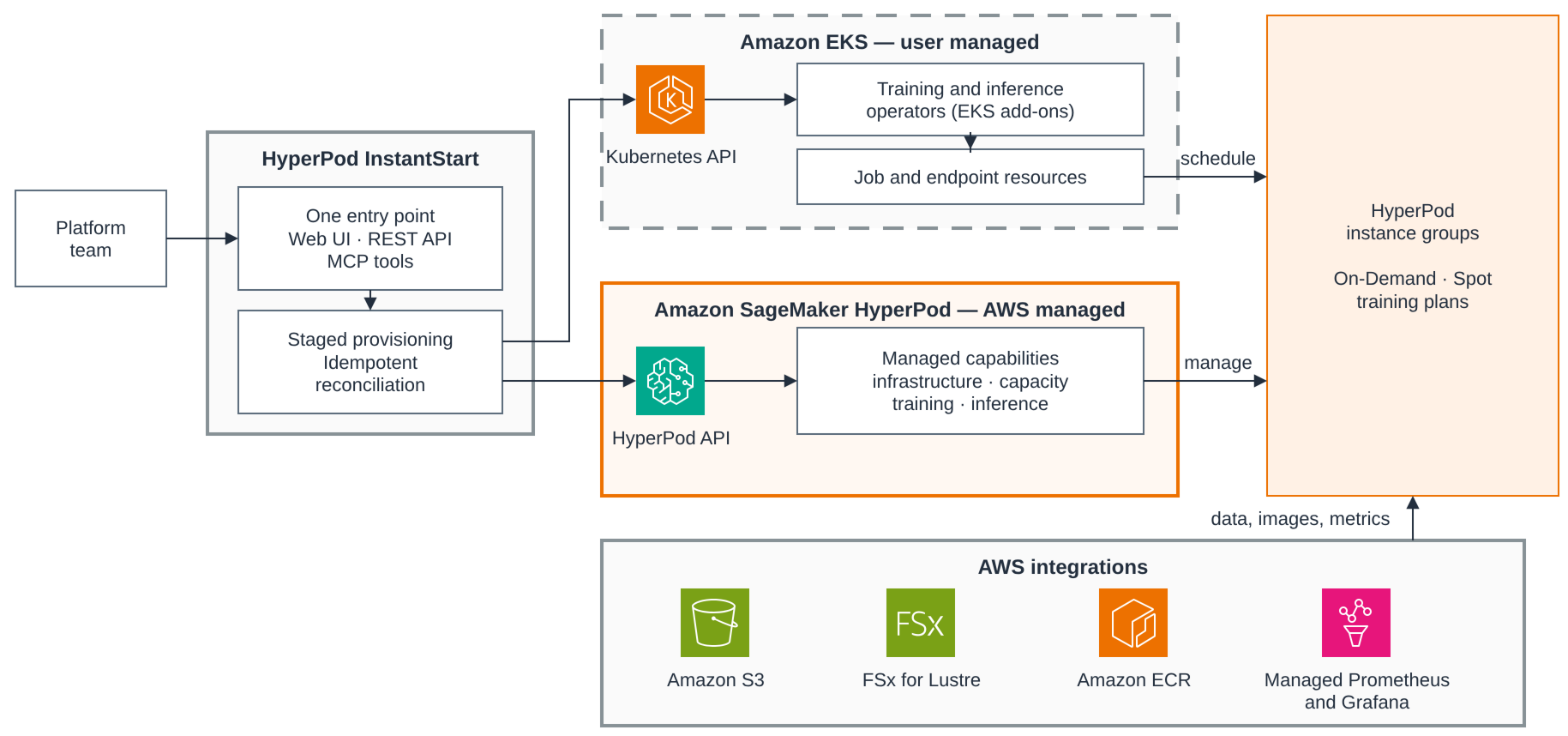
- Why the design choices map cleanly onto Amazon SageMaker HyperPod with Amazon Elastic Kubernetes Service (Amazon EKS).
- Cluster and shared multi-terabyte storage layer setup.
- Distributed post-training for three representative workloads, with a complete end-to-end walkthrough of the robot-policy stage on a public DROID dataset.
The accompanying repository contains the manifests and configuration files for each stage. You can find the runnable code, including the infrastructure templates and job manifests that turn this design into a working cluster, in the awsome-distributed-ai GitHub repository.
Running the loop is a capacity commitment. Acquiring GPUs stage by stage adds variability at this scale: availability and lead times can vary, and the capacity that you do get might land in an Availability Zone or AWS Region away from your data. Committing capacity to the whole loop avoids that churn, whether through a flexible training plan for a bounded campaign or a capacity reservation for an open-ended one. Because you pay for that capacity whether or not the pipeline is making progress on it, the metric that governs cost is not the peak throughput of any one job. It is GPU goodput: the useful pipeline progress per reserved GPU-hour across the whole loop.
Physical AI pipelines often provision separate GPU capacity for each stage: one set of nodes to generate synthetic data, another to post-train, another to evaluate, each with its own lifecycle to stand up and tear down. NVIDIA Cosmos 3 makes that unnecessary. As an open omnimodal world foundation model, Cosmos 3 treats video, image, action, and sound as a single token stream. It runs the same transformer trunk in three modes: a forward-dynamics world model for synthetic video generation, an inverse-dynamics action labeler, and a deployable action policy. Because one model family covers generation, post-training, and evaluation, those stages become three workloads scheduled onto one persistent, resilient GPU node pool under a single cluster control plane. It’s time-shared capacity rather than a separate pool per stage. NVIDIA released it under the Linux Foundation’s OpenMDW-1.1 license, and describes the architecture in the Cosmos 3 technical report.
1. How Cosmos 3 works
A common pattern for world models is to pair a diffusion-transformer video generator with a separate vision-language model that provides text conditioning. Cosmos 3 takes a different approach: one trunk that handles both, integrated at every layer. That integration is what makes it useful as the engine of an end-to-end Physical AI model factory. Three architectural choices define it:
- One token stream. Every modality feeds into a single shared sequence, so one model can both read and generate across modalities. Images the model reads for understanding, pixels it generates, and a compact per-embodiment vector of pose deltas and grasp state each get their own encoder. A vision transformer (ViT) handles image understanding while a frozen Wan2.2 video variational autoencoder (VAE) handles pixel generation. That one action vector is what lets the same model drive both an AV and a robot arm. The sequence puts an autoregressive (AR) zone (the text and vision it reads) ahead of a diffusion zone (the video, audio, and action it produces).
- Two experts, joined at every layer (MoT). Each layer runs a reasoner that predicts the next token and a generator that denoises video, audio, and actions. Dual-stream attention joins them so generation stays grounded in the reasoner’s output at every layer, not only once at the end. The common alternative bolts a diffusion transformer (DiT) onto a vision-language model (VLM) and cross-attends to its final output once. Cosmos 3 grounds generation in the reasoner all the way down.
- Asymmetric at inference. Training and deployment do not run the same amount of work. Training runs the full denoising schedule and decodes video back to pixels, because that predicted video is part of the loss. On the robot, the same model runs a few denoise steps and skips video decoding entirely. The video latents are still produced internally to ground the action, but only the action tokens are decoded into the joint positions the robot executes.
The following diagram shows the first two choices in one view: the shared token stream and the two experts joined by attention. The autoregressive (AR) subsequence (text and the vision tokens the model reads to understand) and the diffusion-model (DM) subsequence (the video, audio, and action tokens it generates) run through the shared Reasoner and Generator towers. The attention mask on the right shows how the two experts differ: DM queries attend over both AR and DM keys (full attention), while AR queries stay causal and never see the diffusion tokens.
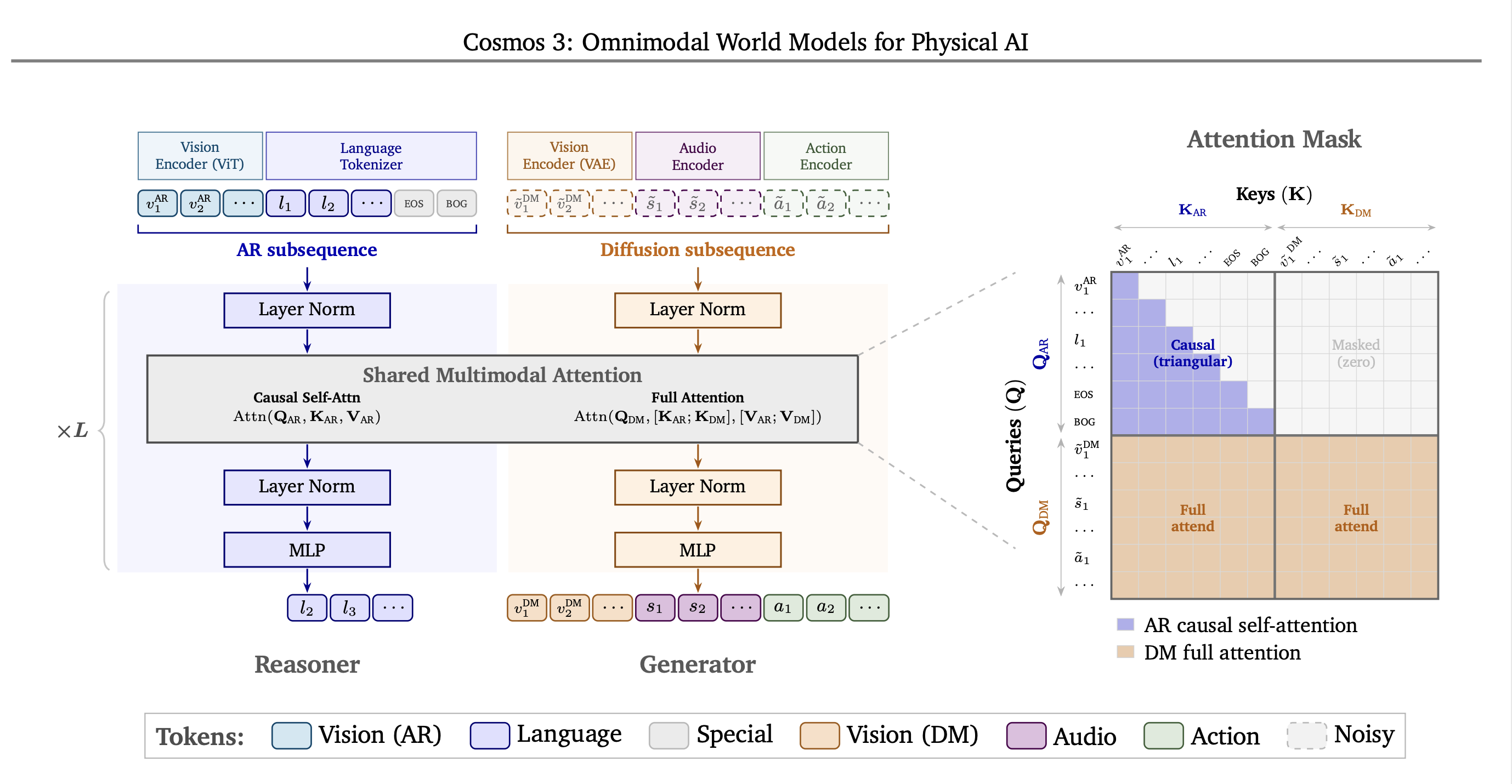
Figure 1: The Cosmos 3 shared token stream and its two experts joined by per-layer attention
(source: Cosmos 3: Omnimodal World Models for Physical AI)
Three action modes, one architecture
The mid-trained base checkpoint runs three jobs by changing which tokens start as noise. Post-training then specializes a checkpoint to a single mode and control frequency.
- Forward dynamics (world model). Actions clean, video noisy. “Given this frame and this action, what comes next?” This is the synthetic-data engine, fanned out to generate long-tail driving scenes or rare manipulation interactions that real collection cannot reach affordably.
- Inverse dynamics (action labeler). Video clean, action noisy. “Given these two frames, what action caused the change?” Converts unlabeled video (raw teleoperation recordings, third-person robot video, YouTube driving footage) into action-labeled training data.
- Policy (the deployed robot). Both noisy, conditioned on 3-view image plus proprioception. It outputs 32 future joint positions, with predicted video frames as a byproduct that grounds the action prediction.
The model family has two tiers: Cosmos3-Nano (16B parameters, on a dense 8B parameter Qwen3-VL backbone) and Cosmos3-Super (64B parameters, on a dense 32B parameter Qwen3-VL backbone). Task variants such as Cosmos3-Nano-Policy-DROID build on these tiers. NVIDIA also released Cosmos3-Edge, a compact 4B tier for on-device deployment (benchmarked on Jetson Thor and Orin). Edge shares the same physical-world pretraining data as Nano and Super but is built on a dense ~2B backbone trained from scratch rather than initialized from Qwen3-VL, so it is a separate weight lineage: you post-train Edge directly for the target hardware rather than shrinking a Nano checkpoint into it.
The following diagram shows the three modes side by side, with solid boxes for clean (known) tokens and dashed boxes for noisy tokens the model denoises. Forward dynamics keep the actions and the current frame clean and denoises future video. Inverse dynamics keep the video clean and denoises the actions. The policy sees only the first frame clean and denoises the actions the robot will execute. The same architecture runs all three, and only the pattern of clean versus noisy tokens changes. In the base checkpoint all three modes are available; a post-trained variant such as Cosmos3-Nano-Policy-DROID is specialized to policy mode at 15 Hz with a 32-step horizon.
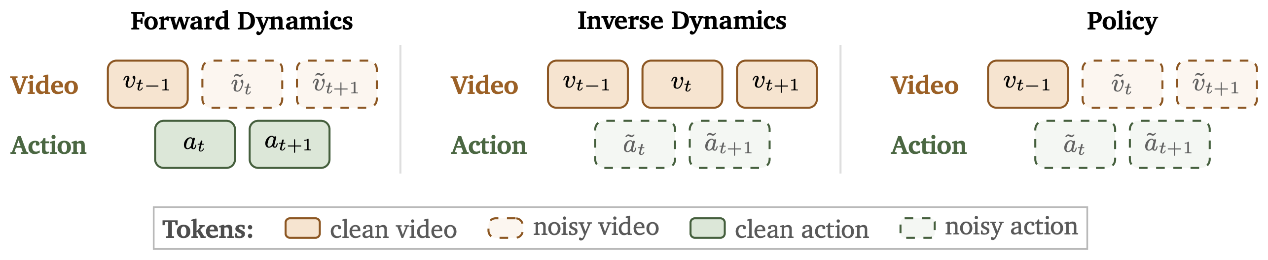
Figure 2: The three action modes of one checkpoint, set by which tokens start as noise
(source: Cosmos 3: Omnimodal World Models for Physical AI)
2. From one model to a perpetual model factory
A team producing a robot or AV does not run one fine-tuning workload. It runs a loop: ingest real data, curate it, augment it with synthetic data, post-train, evaluate in a closed-loop simulation, deploy the policy, collect more data, and repeat.
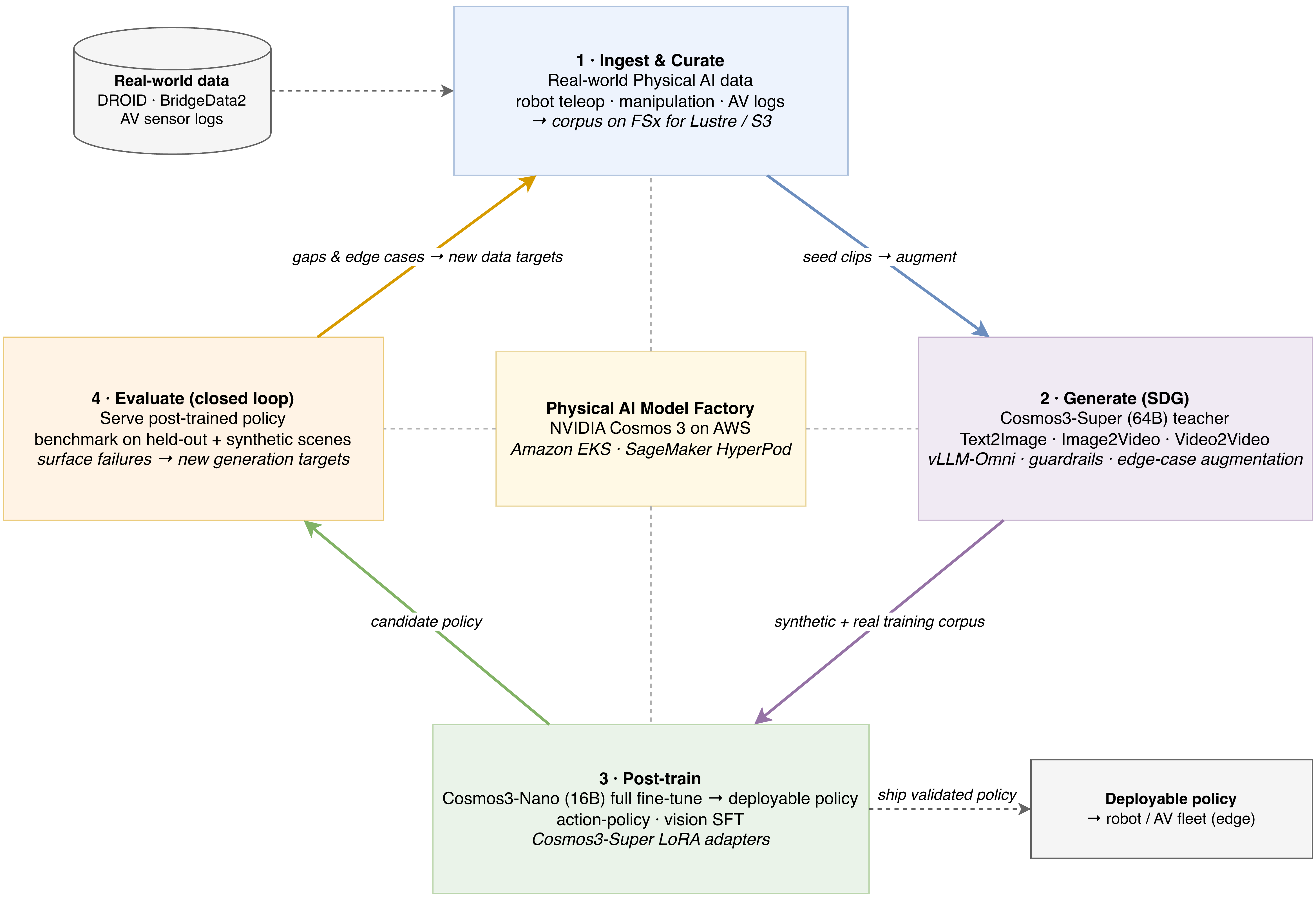
Figure 3: The Physical AI model factory as a four-stage flywheel
The loop has four stages. (1) Ingest and curate real-world Physical AI data (DROID, BridgeData2, AV sensor logs) into a shared corpus on Amazon Simple Storage Service (Amazon S3) and Amazon FSx for Lustre. (2) A Cosmos3-Super teacher generates synthetic data to augment that corpus. (3) The combined synthetic and real corpus post-trains a deployable Cosmos3-Nano policy, with vision fine-tuning applied across both the Nano and Super tiers. (4) The policy is evaluated in closed-loop simulation, and its failures become new generation targets that re-enter the corpus for the next round.
Ideally, that loop doesn’t stop, with each stage running again as new data arrives. That cadence makes the cost driver GPU goodput (useful pipeline progress per reserved GPU-hour) rather than the peak throughput of any one job. Goodput is highest when the stages share one pool, so few GPU-hours are lost re-provisioning or moving data between separate clusters. Cosmos 3 makes that possible: it unifies three model classes (a world-sim generator, a policy, a perception model) into one model running in different modes. To support that flywheel, the cluster underneath must match that shape: one persistent pool on one control plane, instead of a disparate compute environment per job.
Amazon SageMaker HyperPod on Amazon EKS delivers exactly that shape. Each of the architectural choices behind Cosmos 3 creates a concrete cluster demand. The single token stream and the 64B MoT structure make training a long-sequence, multi-node job that needs a low-latency interconnect. The train-versus-inference asymmetry keeps generation, post-training, and evaluation on one model and one storage layer, so they can time-share one committed pool of capacity rather than fragmenting it stage by stage. Running the flywheel continuously requires capacity that is reserved and continuously monitored. Four Amazon SageMaker HyperPod properties answer those demands in turn:
- One cluster for all stages. Because Amazon SageMaker HyperPod orchestrates the cluster with EKS, the three engines of the loop run as ordinary Kubernetes workloads on a single shared GPU pool. Generation runs on the vLLM-Omni server, post-training on cosmos-framework under torchrun (Fully Sharded Data Parallel (FSDP2) plus Ulysses context parallelism), and evaluation on a single-GPU policy server. They also share one storage layer. An Amazon FSx for Lustre file system, accessed over Elastic Fabric Adapter (EFA), backed by an Amazon S3 bucket through a data repository association (DRA), mounts once and serves all three stages from the same path. Generation writes synthetic clips, post-training reads them, and the policy server loads its checkpoint off the same volume. There are no re-provisioning steps or terabyte-scale data migrations between stages, and Region-locked AV data stays in one in-Region cluster.
- Health-checked, auto-recovering capacity. A continuous loop wants capacity that is already provisioned and actively monitored: generation is bursty and dominates GPU-hours, and post-training runs for days across many nodes. Amazon SageMaker HyperPod continuously detects faulty nodes and reboots or replaces them automatically, and you can commit that capacity ahead of time with flexible training plans. Its managed job auto-resume then turns a worker failure into a bounded recovery. The Kubeflow PyTorchJob recreates the pod gang, NCCL re-forms, and cosmos-framework resumes from the latest PyTorch Distributed Checkpoint (DCP). A node failure therefore costs at most one checkpoint interval of redone work plus the node-replacement and reschedule latency, rather than a lost run.
- EFA already wired for multi-node NCCL. The long sequences that Cosmos 3 packs together for training (video latents plus text plus action, tens of thousands of tokens each) push the 64B tier into context parallelism on top of FSDP2. Every layer issues cross-node collectives. Standing that up by hand is the usual multi-node time sink: matching the EFA stack, the NCCL plugin, and the exact torch and NCCL versions the cosmos-framework pins. Amazon SageMaker HyperPod ships it pre-configured, and when paired with an AWS Deep Learning Containers (DLC) image, whose torch and aws-ofi-nccl versions match what the framework pins, NCCL over EFA is configured to work out of the box.
- Optional: task governance for many embodiments. If the factory serves several robot types or AV variants at once, Amazon SageMaker HyperPod task governance (built on Kueue) carves the pool into namespace-scoped queues with quotas, priorities, and preemptions. Dozens of heterogeneous jobs then share one capacity reservation instead of contending for it ad hoc, which raises goodput by keeping otherwise-idle GPUs busy across projects. A single-embodiment program can skip it, but task governance pays off once many jobs compete for the same pool.
The choice between Amazon SageMaker HyperPod and a lighter option comes down to the unit of work. A one-shot fine-tuning workload does not necessarily need the resilience and persistence of an Amazon SageMaker HyperPod cluster. An ephemeral managed training job (for example, an Amazon SageMaker AI training job) suffices, because a short run rarely hits a node failure. Amazon SageMaker HyperPod is well-suited for the sustained Cosmos 3 flywheel, where generation runs continuously, post-training is multi-node and long-running, evaluation is co-located on the same storage layer, and failures are statistically frequent.
3. What we are building
The solution post-trains three representative workloads, each a stage of the flywheel, and exercises the generation and evaluation stages end-to-end. All three run end-to-end on p5en.48xlarge (8x NVIDIA H200 GPUs) nodes with real checkpoints. The three are a robot-manipulation policy and two vision-perception fine-tuning workloads.
| Workload | Stage | Model | What it exercises |
| Robot policy (DROID) | Post-train (policy) | Cosmos3-Nano (~16B) | Action-policy post-training on a public LeRobot v3 dataset (droid_policy.toml). The lightest per-step workload |
| Vision Supervised Fine-Tuning (SFT) | Post-train (perception) | Cosmos3-Nano (~16B) | Video plus caption SFT (vision_sft_nano.toml). Substantially heavier per step than the policy workload |
| Vision Low-Rank Adaptation (LoRA) | Post-train (perception) | Cosmos3-Super (~64B) | LoRA fine-tuning of the 64B model with context parallelism (vision_sft_super.toml). The heaviest per-step workload |
Although AV post-training is not specifically covered here, Cosmos3’s base models were trained on a public synthetic-driving corpus (SDG-DriveSim, the nvidia/PhysicalAI-WorldModel-Synthetic-Autonomous-Driving-Scenarios dataset on Hugging Face). Its per-embodiment action projection is designed to extend to an AV ego-pose action space, so the same recipe and cluster setup covered in this post applies to AV post-training too.
The training stack is NVIDIA’s cosmos-framework, run with no forks or source edits to the framework package, so upstream updates drop in cleanly. It trains with FSDP2 and scales to hybrid sharded data parallelism (HSDP) and context parallelism as sequence length and node count grow. Section 6.2 covers how those parallelism choices are set per tier.
This guide uses p5en.48xlarge as the reference instance type throughout. Rather than publishing a cross-instance ranking, we give you a goodput methodology you can run on your own hardware (Section 7). It is built on per-step time, GPU saturation, and a configurable Model FLOPs Utilization (MFU). With it you can size your chosen platform, including the NVIDIA Blackwell platform (B200, B300, and rack-scale GB200/GB300 NVL72), against your own measurements.
4. Cluster setup on SageMaker HyperPod EKS
Setting up the cluster breaks down into satisfying the prerequisites, enabling NCCL over EFA, turning on deep health checks and auto-recovery, choosing a base training image, and staging and validating the result.
4.1 Prerequisites
You can satisfy most of these prerequisites with the Amazon SageMaker HyperPod-EKS Terraform modules. These modules provision the EKS-orchestrated Amazon SageMaker HyperPod cluster, the virtual private cloud (VPC) and EFA-enabled security groups, the Amazon FSx for Lustre file system and CSI driver, the Kubeflow training operator, and the observability add-on. If you prefer, you can also use the Amazon SageMaker AI console to create these resources using AWS CloudFormation. Alternatively, you can bring your own equivalents.
You need the following in place before the first job runs:
- Cluster. An Amazon SageMaker HyperPod cluster orchestrated by Amazon EKS, with a GPU instance group of p5en.48xlarge nodes in a single Availability Zone (see Creating an Amazon SageMaker HyperPod cluster with Amazon EKS orchestration). At this scale, GPU capacity is the binding constraint: p5en is rarely available on demand, so plan on a flexible training plan or a capacity reservation to secure the nodes.
- Service quota. Because GPU capacity constrains availability, a sufficient service quota for the chosen instance type in the target Region, requested through AWS Service Quotas before you scale up the cluster.
- Job submission. kubectl configured against the cluster and the Kubeflow Training Operator installed, so that PyTorchJob custom resources are recognized.
- Storage. The FSx for Lustre CSI driver installed and an Amazon FSx for Lustre file system attached in the same VPC and subnet as the GPU nodes. The Terraform modules provision both when you turn on the FSx module, or you can attach an existing file system.
- Credentials. A Hugging Face read token with the nvidia/Cosmos-Guardrail1 license accepted on the token’s account, stored as a Kubernetes secret named hf-token, because the generation and policy-serving paths pull this gated guardrail repository at startup.
4.2 Enabling NCCL over EFA
EFA gives NCCL a kernel-bypass, remote direct memory access (RDMA) capable transport for multi-node collectives, and each p5en.48xlarge node advertises 16 EFA Network Interface Cards (NICs). On Amazon SageMaker HyperPod EKS the EFA drivers (from the Deep Learning AMI) and the EFA device plugin (pre-installed by the HyperPod service) are already in place. The pod spec only requests vpc.amazonaws.com/efa resources alongside the GPUs (see the sample manifests). The training image must carry an aws-ofi-nccl plugin built against the same NCCL version the framework uses, which is exactly why this sample builds on the AWS DLC (Section 4.4).
EFA being present on the hardware is not the same as NCCL actually using it, so verify the transport rather than assume it. The training manifest runs a short diagnostic preamble before training starts, and with NCCL debug logging on, a healthy multi-node run reports EFA with GPUDirect RDMA as the selected transport. A fallback to TCP appears as NET/Socket in the logs, meaning the collectives are running over the wrong transport. To validate the interconnect end-to-end before a real run, run a standard multi-node NCCL test (for example, all_reduce_perf) and confirm the achieved bus bandwidth (see the NCCL tests guide). For the exact diagnostic commands and the full log signature, see the repository README.
4.3 Deep health checks and auto-recovery
A per-node health-monitoring agent continuously runs basic, passive checks (DCGM policy violations, nvidia-smi errors, GPU-count validation), while deep health checks (DCGM level-4 diagnostics and NCCL/EFA benchmarks) run when nodes join or the cluster is updated. When you turn on automatic node recovery, a fault from any of these sources triggers Amazon SageMaker HyperPod to reboot or replace the faulty instance, and auto-resume restarts the job from the last checkpoint once the replacement is ready.
4.4 Choosing the base training image
Getting distributed training to run across nodes can consume a surprising amount of setup time, so it is worth treating the base-image choice as a deliberate decision rather than an assumption. The choice hinges on one question: do NCCL collectives ride EFA across nodes, and do the cosmos-framework pinned CUDA wheels load? The framework’s virtual environment (venv) pins torch==2.10.0+cu130 (CUDA 13), and its CUDA wheels (flash-attn, transformer-engine, natten) are published for CPython 3.13 only. These pins drive the base-image choice in two ways: the image’s NCCL must match the torch wheel’s bundled NCCL for EFA to work, and the image must provide a CPython 3.13 environment for the wheels to install at all.
A mismatched base image may block multi-node. A general-purpose GPU PyTorch base image can validate single-node yet fail cross-node NCCL over EFA at initialization (for example, fi_getinfo() No data available) even when EFA itself is fully functional. The root cause is a version-matrix mismatch. The cosmos-framework venv’s torch bundles a specific NCCL (here, 2.28.9), but if the base image’s bundled aws-ofi-nccl plugin was built against a different NCCL, the plugin and the runtime don’t line up. Setting NCCL_NET_PLUGIN=none sidesteps the error, but only by dropping cross-node traffic onto TCP instead of EFA, a non-starter for multi-node performance.
A version-matched AWS Deep Learning Containers image removes this work. The AWS Deep Learning Containers (DLC) for PyTorch ships torch 2.10.0+cu130, an exact match to the cosmos-framework pin. It also bundles an AWS tuned, version-matched EFA stack (EFA 1.47.0, libfabric 2.4, aws-ofi-nccl 1.18.0, GDRCopy 2.5.1). Because the DLC ships the same torch wheel the venv installs, NCCL and the aws-ofi-nccl build in the DLC line up. Multi-node EFA is then configured to work without a plugin rebuild or a version mismatch to work around.
Two further build-time issues surfaced in the DROID video-decode path on the DLC: an FFmpeg version too old for torchcodec, and a missing shared libpython. Both are packaging problems with clean fixes baked into the Dockerfile in the accompanying repository.
In short, pick the base image by cosmos-framework version compatibility and verified NCCL over EFA, not by brand or familiarity. For this framework version, the version-matched AWS DLC can be a lower-effort path.
4.5 Staging and validation
With the base image chosen and the prerequisite cluster in place, you stage the image and storage and validate the result before running a workload. Each step is backed by code in the accompanying repository, so you run templates rather than hand-assemble resources.
Build and push the training image to Amazon Elastic Container Registry (Amazon ECR), and apply the storage class and the optional Amazon S3 data repository association so datasets and base checkpoints hydrate into /fsx on first access:
Before submitting a job, you validate that the cluster is ready: confirm that every GPU node shows Ready and the Kubeflow training-operator pod shows Running.
With provisioning and validation done, Section 6.1 walks through preparing data, launching the robot-policy job, monitoring it, and validating its output, and Section 10 covers how to tear the workloads and cluster back down when you’re finished.
5. Wiring the storage layer
The flywheel moves multi-terabyte datasets between stages, so the storage layer is a first-class design decision rather than an afterthought.
Staging: Hugging Face to S3 to FSx for Lustre. Datasets and base checkpoints stage from Hugging Face into an in-Region Amazon S3 bucket, which is then attached to an FSx for Lustre filesystem through a DRA. FSx for Lustre presents one POSIX namespace at /fsx to each pod, and the DRA lazily loads objects from S3 on first access or preloads them on demand.
Two I/O regimes. The workloads don’t stress storage the same way, so it helps to treat them as two distinct regimes. The robot-policy data (the LeRobot/DROID dataset) is a metadata and small-file regime: many small Parquet shards and short video clips, where request rate and latency matter more than raw bandwidth. The video SFT data is a bandwidth and large-file regime, where sustained throughput dominates. Because the two regimes pull in different directions, the right backend depends on the access pattern, not on a single best-choice verdict. Both regimes are served from one FSx for Lustre filesystem here. Per-directory Lustre tuning (stripe count and size, progressive file layouts, and client-side read-ahead) is a further optimization you can layer on per access pattern rather than something this sample presets.
FSx for Lustre plus EFA, with cold versus warm tradeoffs. Provision an EFA-enabled PERSISTENT_2 FSx for Lustre file system sized for a throughput target (1000 MBps/TiB), because capacity governs the aggregate throughput ceiling: the sample’s 9.6 TiB filesystem tops out around 9.4 GB/s aggregate. EFA is what lifts the per-client ceiling. A non-EFA file system caps at 100 Gbps per client instance, whereas an EFA-enabled file system reaches 700 Gbps per client over EFA. With GPUDirect Storage on EFA-enabled NVIDIA GPU instances such as p5en, it reaches up to 1200 Gbps. AWS recommends enabling EFA for any file system above 10 GBps for this reason. Treat these as documented ceilings rather than measured throughput: benchmark with fio (installed in the training image) on your own cluster, and note that traffic to a single object storage server (OST) caps at 5 Gbps, so a high per-client rate requires striping across many OSTs. The backends also differ most on raw throughput at first touch: local NVMe is fastest, FSx for Lustre sits below it, and a cold read from Amazon S3 is slower still. That gap is a cold-start and first-touch cost. After a working set is page-cache warm, training reads are served from RAM, so the backend ceases to be the bottleneck. Backend choice therefore matters for cold-start and for working sets larger than RAM, not for warm reuse of a cache-resident dataset. The cosmos-framework dataloader reinforces this: background workers prefetch and decode upcoming batches while the GPU computes the current step, so once the working set is warm, steps stay compute-bound rather than I/O-bound.
6. Launching distributed post-training
This section runs the robot-policy stage end to end, then explains how the job maps onto Kubernetes, how parallelism is configured on H200, and how resilient checkpointing works.
6.1 Running the robot-policy stage end to end
Post-training the robot-policy workload comes down to a short sequence: prepare data and the base checkpoint, launch the distributed job, monitor it, and validate the output. The walkthrough uses the SageMaker HyperPod manifests, which render their environment variables with envsubst before kubectl applies them. The subsections that follow explain the machinery behind each step.
You first prepare data and the base checkpoint. Point the Amazon FSx for Lustre DRA at the Amazon S3 bucket holding the public DROID dataset, so the dataset hydrates into /fsx on first read. The Hugging Face-released checkpoint ships as Diffusers/safetensors, so you convert it once to the DCP format the cosmos-framework loads (a CPU job is fine, though the 64B Super needs several hundred GB of RAM):
You then launch the distributed job by rendering and applying its manifest, which wires the image, the /fsx volume, and the torchrun launch into a Kubeflow PyTorchJob (Section 6.2):
You monitor progress in two ways. kubectl shows scheduling and pod health, and the goodput dashboard from Section 7 shows loss, per-step time, and GPU saturation as the run proceeds:
You validate output by confirming the run writes DCP checkpoints to $IMAGINAIRE_OUTPUT_ROOT on /fsx at the configured interval, and that training loss on the dashboard trends down as step time holds steady. Because the checkpoint lands on the shared volume, the evaluation server in Section 9 can load it directly, which closes the loop.
6.2 How the job maps onto Kubernetes
The manifest launched in Section 6.1 wraps torchrun in a Kubeflow PyTorchJob, one primary replica and N−1 worker replicas for an N-node run. The PyTorchJob controller injects the standard PyTorch rendezvous variables (coordinator address and port, per-pod rank, and world size) into each pod, and torchrun then spawns one process per GPU to form the global process group over EFA. On a 2-node p5en run this is 16 ranks across 2 nodes.
6.3 Parallelism configuration on H200
The three post-training workloads split by tier. The 16B Nano is fully fine-tuned into the deployable policy, because it is the model that ships to the robot and is small enough that full-parameter training is affordable. The 64B Super is the synthetic-data generator, and it is adapted with LoRA rather than fully retrained: you rarely need to relearn a 64B teacher, only shift it toward your domain (your cameras, lighting, object classes, or scenario mix). Freezing the backbone and training rank-16 adapters collapses optimizer and exponential-moving-average (EMA) memory, shrinks checkpoints from a 64B snapshot to megabytes of adapter tensors, and lets one frozen Super base serve many domains by swapping adapters. All of this raises goodput on the large tier.
Those tiers also drive the parallelism strategy, with the H200’s 141 GB of high-bandwidth memory (HBM) as the lever for minimizing communication. More HBM per GPU means less aggressive sharding and fewer collectives per step. The Nano workloads run pure FSDP2 with a shard degree set to the world size. Super adds context parallelism degree 2 on top of FSDP2, because the long-packed sequences make attention activation memory the limiter. Ulysses context parallelism splits the sequence across GPUs with only a couple of all-to-alls per attention layer. At larger node counts, set the replicate degree above 1 to switch to HSDP when cross-cluster all-gather traffic becomes the bottleneck.
The sample also applies two small runtime patches at import time rather than editing the framework: a guard against an empty-shard edge case in gradient-norm monitoring at high rank counts, and the OpenTelemetry metrics bridge covered in Section 7. Both are applied from the sample, so upstream framework updates still drop in cleanly.
6.4 Resilient checkpointing
The cosmos-framework writes checkpoints as PyTorch Distributed Checkpoint (DCP), and the action-policy checkpoint behavior is preset in the checkpoint block of the action_policy_public_lerobot experiment. Three settings there matter for a resilient warm-start:
dcp_async_mode_enabled=False, so saves are synchronous by default. Set it toTruefor async DCP, which keeps steady-state checkpoint stall negligible while bounding lost work on failure.strict_resume=False, so a freshly initialized action head (or LoRA adapters) can initialize while the rest of the model warm-starts from the converted base checkpoint (Section 6.1).keys_to_skip_loadinglists the tensors not expected during load (the action heads and the base model’s EMA weights), so they initialize fresh rather than erroring out.
A fourth setting, ckpt_type, defaults to dcp in the same experiment but is meant to be overridden per run (for example, dummy for a smoke test). Changing any of the preceding three settings means editing the experiment config, not passing a runtime flag.
Async DCP saves pin roughly model-size in host shared memory, so set the pod’s /dev/shm volume sizeLimit generously. For example, 256Gi works well since P5en has roughly 2 TiB of host memory. At 64Gi the save can throw an out of memory (OOM) error.
Combined with HyperPod auto-resume, a pod restart or node replacement continues from the last checkpoint automatically. The training manifest also checks for an existing checkpoint at startup and resumes from it rather than starting from scratch.
7. Measuring what matters: A goodput methodology you can run
This section gives you a metrics setup you can reproduce on your own cluster. It builds on the Amazon SageMaker HyperPod EKS observability add-on and unifies GPU telemetry and cosmos-framework training metrics in one Amazon Managed Grafana pane, using a dashboard and bridge that ship with the accompanying repository. The dashboard is an importable Grafana model, cosmos3-goodput-dashboard.json. To load it, open your Grafana workspace, choose Dashboards, New, Import, and upload the file, as described in the observability README.
Infrastructure and GPU metrics, by default. Streaming multiprocessor (SM) and HBM utilization, NCCL and EFA traffic, and node health all flow into Amazon Managed Service for Prometheus through the DCGM exporter and node exporters, with no custom instrumentation. The Amazon SageMaker HyperPod observability add-on provides the cluster, node, and job views without additional configuration, rendered in Grafana alongside the cosmos-framework metrics.
Cosmos framework metrics, bridged into the native stack. The cosmos-framework emits loss, per-step timers, MFU, gradient norm, and sequence-packing statistics through its callbacks, which default to Weights & Biases (W&B). To land these in the same Prometheus workspace as the GPU metrics with no W&B dependency, the repository ships a small OpenTelemetry Protocol (OTLP) bridge. The bridge mirrors those framework scalars to the Amazon SageMaker HyperPod observability add-on’s in-cluster OTLP collector (the hyperpod-otel-collector service, reached over gRPC). It also adds a Cosmos-specific MFU callback that exposes MFU against a peak-FLOPS constant you configure. To turn it on, set one environment variable on the training pod: set OTEL_EXPORTER_OTLP_ENDPOINT to the observability add-on’s in-cluster OTLP endpoint (http://hyperpod-otel-collector.hyperpod-observability.svc:4317). Leaving it unset keeps the default path unchanged. The repository also ships the Grafana dashboard and OTLP bridge that render both metric sources together.
The following two panes are an illustrative capture from a single run, not a performance result to read numbers from. The first pane is the cosmos-framework trainer view. It shows training loss, step time, achieved TFLOPS per GPU, Model FLOPs Utilization (here computed against the framework’s default per-GPU peak), iteration throughput, gradient norm, and sequence-packing token lengths, all bridged from the framework callbacks.
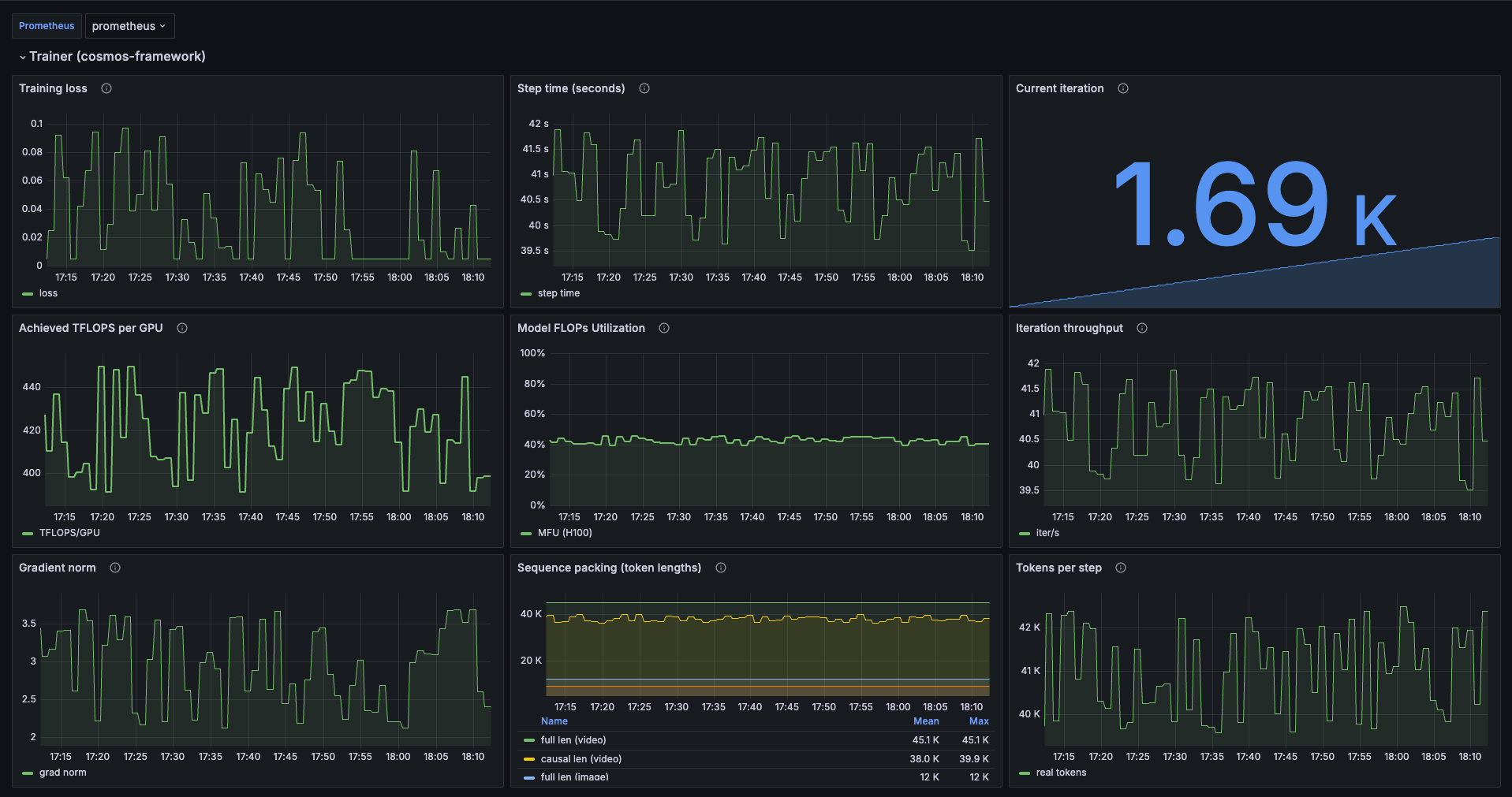
Figure 4: The cosmos-framework trainer pane, bridged from the framework callbacks
The second pane is the GPU and infrastructure view from the Amazon SageMaker HyperPod observability add-on (using the DCGM exporter): graphics-engine-active, GPU utilization, framebuffer (HBM) used, and GPU power, reported per GPU so an idle or under-driven device is immediately visible.
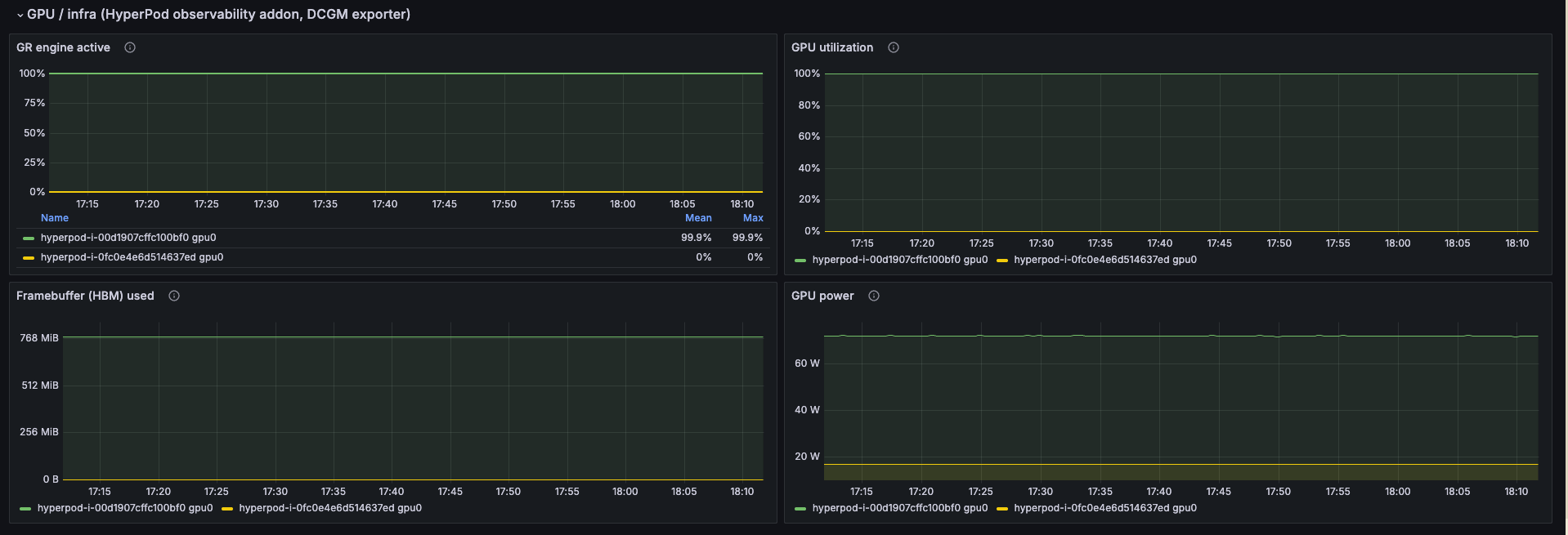
Figure 5: The GPU and infrastructure pane from the observability add-on, using the DCGM exporter
This setup surfaces two layers of signal, as methodology rather than a published score:
- Micro layer: Per-GPU saturation and step efficiency. DCGM graphics-engine-active and HBM utilization come straight from the observability add-on as directly measured hardware signals. The cosmos-framework callbacks add achieved TFLOPS per GPU, iteration throughput, gradient norm, and sequence-packing token lengths. MFU is also surfaced, computed against a configurable per-GPU peak-FLOPS constant you set for your accelerator and precision.
- Macro layer: Goodput framing. Combine the micro-layer saturation with the goodput fraction to reason about effective utilization across the whole flywheel, rather than the peak throughput of any one step. The goodput fraction is the share of GPU-hours spent on useful forward progress, after initialization and scheduling, checkpoint stall, and restart and recovery.
7.1 How fault recovery works
On this stack, a single worker-pod or node failure during a long run resolves without manual intervention, and the path is worth tracing because it determines the cost of a failure. After a node fault, the Amazon SageMaker HyperPod health monitoring agent detects the bad node, and its node recovery system reboots or replaces it. The PyTorchJob’s managed auto-resume (with the sagemaker.amazonaws.com/enable-job-auto-resume annotation) then recreates the pod gang onto healthy capacity. torchrun re-rendezvous, and cosmos-framework auto-resumes from the latest checkpoint. Training continues from the last checkpoint rather than from scratch.
Recovery decomposes into two buckets: (b1) node replacement and pod reschedule, and (b2) checkpoint reload plus catch-up to the failure point. Although b2 is framework-level and behaves the same across platforms, the node auto-replacement and job auto-resume of Amazon SageMaker HyperPod address the b1 portion, the part that otherwise requires a human to detect, replace, and restart. With b1 automated and b2 bounded by the checkpoint interval, a failure costs at most one checkpoint interval of redone work plus the b1 reschedule latency, rather than a lost run, and it is the basis for optimizing checkpoint interval sizing.
7.2 Picking the goodput-optimal checkpoint interval
The checkpoint interval is how often training saves its state. Save too rarely and a failure throws away a lot of work. Save too often and the saves themselves eat into useful compute. The cosmos-framework checkpoints in an async mode: the GPUs copy the model state to host memory quickly, and training continues while the write to FSx finishes in the background. The steady-state cost of a save is therefore small, and a single-worker failure costs roughly one checkpoint interval of lost work plus the time to reschedule and reload.
There is a known-optimal interval that balances these two costs, given by the Young/Daly formula: interval ≈ √(2 × C × MTBF), where C is your checkpoint save cost and MTBF is the mean time between failures. Both inputs are things you measure on your own cluster rather than guess. For a published anchor, Meta’s Llama 3 405B pre-training saw one interruption roughly every three hours on 16,384 H100 GPUs. Treat it as an order-of-magnitude illustration, not a number to reuse, since it is H100 at far larger scale than this sample’s p5en cluster. C is the save duration you can read from the cosmos-framework step metrics. MTBF is the average run-time between node failures observed across your fleet, an estimate that sharpens as you accumulate run history.
For example, with a 30-second save cost and a 24-hour MTBF (86,400 s), the optimal interval is √(2 × 30 × 86,400) ≈ 2,300 s, or about every 40 minutes. At that interval, the checkpoint overhead works out to roughly 30 s of saving every 2,300 s, on the order of 1% of wall-clock, which is the goodput the interval is tuned to protect. Plug in your own C and MTBF to get the interval that maximizes goodput on your cluster, and re-derive it if either changes. Note MTBF is a fleet-level quantity: for N nodes it is roughly the per-node MTBF divided by N, so a 1024-GPU (128-node) cluster fails far more often than a 16-GPU (2-node) cluster and needs a correspondingly shorter interval. Scale the per-node figure by your node count before solving.
8. Findings and best practices
These findings are deliberately relative and regime-based (which workload is heaviest, where a backend choice matters), so they hold on your own cluster regardless of the absolute numbers you measure there.
- Measured scaling and saturation. In our runs on p5en (H200) nodes, recorded with the goodput dashboard from Section 7, the Super (64B) LoRA workload held near-flat strong-scaling efficiency as it scaled from 1–4 nodes (8–32 GPUs). It stayed at roughly 0.97–0.99 of linear, with per-step time within about 3% across the ladder. Model FLOPs Utilization, computed against the H200 BF16 peak, landed near 0.50 for the compute-dense Super workload and near 0.24 for the lighter Nano vision workload, in the expected ordering (the larger, more compute-bound model saturates the GPUs more fully). These are relative figures from this setup that should reproduce in shape on comparable hardware, not a leaderboard number.
- Node count and parallelism per workload. Size the node count to your wall-clock target per workload, and let the workload’s per-step cost drive the choice: the 64B Super LoRA tier dominates per-step cost, while the robot-policy workload is the lightest. Because the cosmos-framework packing dataloader holds a fixed per-rank token budget, per-step time, not iterations per hour, is the throughput signal to track as you scale out. The parallelism strategy also shifts from pure FSDP2 toward HSDP as cross-node all-gather traffic grows (Section 6.2).
- Storage by access pattern. The metadata regime favors cold and bulk staging from S3 and warm reuse from local NVMe. The bandwidth regime favors FSx plus EFA as the shared multi-stage plane. The backend matters at cold first-touch, not for warm reuse of a cache-resident dataset.
- What managed resilience buys. Express the return as recovered time and goodput-fraction improvement rather than absolute dollars. Auto-replacement plus auto-resume removes the manual detect-replace-restart loop from every node failure, so the cost of a failure drops to at most one checkpoint interval of redone work plus the node-replacement and reschedule latency.
- When does Amazon SageMaker HyperPod pay off? For a one-shot small fine-tune, an ephemeral managed training job, such as an Amazon SageMaker AI training job that provisions per run and tears down on completion, is sufficient because auto-recovery rarely triggers. Amazon SageMaker HyperPod is well-suited for the sustained, at-scale flywheel: many concurrent jobs, continuous synthetic generation, reserved capacity, and the tens-of-nodes tail where failures are statistically frequent.
9. The flywheel’s other stages: Generation and evaluation
The same cluster, image, and storage layer run the generation and evaluation stages, which closes the loop.
Generation (write-bound). Generation runs on a separate image from training: the official vllm/vllm-omni:cosmos3 engine (a cp312 / vLLM 0.23 stack), not the cosmos-framework DLC training image. It comes up as an OpenAI-compatible server (vllm serve nvidia/Cosmos3-Super --omni) that takes Cosmos3-Super video-to-video (V2V) requests at POST /v1/videos/sync (see the generation manifest). After the server is Ready, port-forward and POST a conditioning clip to get a generated continuation back:
The returned clip is one synthetic example that feeds the next post-training round. This is the stage where AV teams fan out long-tail driving scenarios (the same class of safety-critical corner cases that corpora like SDG-DriveSim target) to augment real fleet data. Generation uses its own parallelism axes, Classifier-Free Guidance (CFG) parallel x Ulysses x HSDP (--cfg-parallel-size, --ulysses-degree, --use-hsdp --hsdp-shard-size), which differ from the training-side FSDP2 + context-parallel knobs and must multiply to the per-node GPU count. The server is single-node, so generation needs no cross-node EFA and scales out as independent servers. Guardrails (nvidia/Cosmos-Guardrail1) are toggled per request (extra_params.guardrails), not through a server flag, and the gated guardrail license must be accepted on the Hugging Face token’s account or startup fails. Delete the generation Job when the batch is done.
Evaluation (latency-bound). A lightweight single-GPU Deployment serves a Cosmos 3 action policy over HTTP for closed-loop evaluation, using the same FSx volume so any checkpoint produced on the cluster is directly available (see the policy-serving manifest). The checkpoint must be a local directory (a bare org/repo Hugging Face id is not resolved by the server), so pre-download or export your own post-trained checkpoint to FSx first. A simulator’s control loop confirms the server is up with GET /info, then posts an observation to POST /predict each step and receives the next action chunk. The request carries the current camera frame and the task prompt:
The server returns the predicted action chunk (the 32 future joint positions described in Section 1), which the simulator applies before sending the next observation. That request/response cycle is the closed loop: the checkpoint that post-training produced is the same one the evaluation server loads off FSx, so a newly trained policy can be evaluated without moving data between clusters.
10. Cost considerations and cleanup
Amazon SageMaker HyperPod is a persistent cluster: instances are billed while they are part of the cluster, FSx for Lustre bills hourly per provisioned capacity, and any serving or visualization pod holds a GPU node for as long as it runs. See the Amazon SageMaker AI and Amazon FSx for Lustre pricing pages for current rates. To pause instance costs between sessions while keeping the cluster configured, scale the GPU instance group to zero, or delete the cluster entirely. See Manage a SageMaker HyperPod cluster. Delete training workloads and the policy-serving Deployment when finished:
Deleting the FSx file system removes its local copy of checkpoints and logs. Data written under the S3 DRA is exported back to the linked bucket and survives, but anything outside that path (or not yet exported) is lost. Confirm your DRA has finished exporting (or download what you want to keep) before deleting and note that the underlying S3 bucket persists independently and bills separately until you delete it too.
11. Conclusion
As Physical AI moves into production, the challenge shifts from a single training run to operating the whole lifecycle continuously and economically. This post described how you can use NVIDIA Cosmos 3 on Amazon SageMaker HyperPod (EKS) as the substrate for that flywheel. That substrate is a persistent, at-scale cluster with one shared storage layer for synthetic generation, post-training of policy and perception models, and closed-loop evaluation, with goodput rather than single-job throughput as the metric that matters. We ran the robot-policy post-training stage on a public DROID dataset, exercised Nano and Super vision fine-tuning across 1–4 nodes, validated multi-node EFA on a version-matched AWS Deep Learning Containers image, and shipped a reproducible goodput dashboard on native observability that unifies cosmos-framework and GPU metrics in one pane. In those runs, the Super workload held near-flat strong-scaling efficiency (roughly 0.97–0.99 of linear) across that range. Because every stage shares the same cluster and storage, a checkpoint that post-training writes to Amazon FSx for Lustre is the same one the evaluation server loads. The synthetic clips that generation produces land on the same volume the next post-training round reads.
This post provides a reference architecture and a reproducible methodology you can point at your own embodiment and data, not a leaderboard you take on faith. To get started, explore the awsome-distributed-ai GitHub repository, use the LeRobotV3ActionDataset recipe as a starting point to adapt to your own dataset, and extend the flywheel to your own robots or vehicles. To learn more, see the NVIDIA Cosmos site, the cosmos-framework repository, and the Amazon SageMaker HyperPod documentation.
About the authors