Data preparation for supervised fine-tuning (SFT) doesn’t end when your dataset is clean and correctly formatted. The harder questions come next. How much data do you actually need? Should you collect more, or select a better subset of what you have? How do you generate high-quality examples when human annotation doesn’t scale? And how do you specialize a model without erasing its general capabilities? This post assumes you have prepared a quality-checked, schema-compliant SFT dataset and are ready to optimize it for training. The first post in this series, Preparing data for supervised fine-tuning Part 1: Formatting and quality, covers that groundwork: the conversational format Amazon Nova expects, the quality checks that catch malformed and low-signal examples, and how to split train and evaluation data without leakage. If your dataset hasn’t been through those steps, start there.
This second post covers four advanced strategies: evaluating data readiness with learning curve analysis, data subset selection and filtering, data augmentation, and data mixing. We reference Amazon Nova customization findings throughout, and the guidance applies to any model you choose.
Data readiness evaluation
After your data is cleaned and formatted, assess whether you have enough signal to train effectively.
Volume and distribution assessment
As a general starting point, plan for roughly 2,000 high-quality training samples for a typical SFT task. Treat this as a ballpark estimate: the right size varies with task difficulty and how far the model’s current behavior is from your goal. A simple format or style change can work with as few as 500 samples, while a complex multi-step reasoning task might require 10,000 or more. Every task and domain has different saturation characteristics.
Before running those experiments, one prerequisite matters more than anything else: a clearly defined evaluation benchmark. This means an evaluation set that’s representative of production traffic, with metrics that reflect what good means for your use case. Most teams find this harder than preparing the training data itself. If you don’t yet have one, build it first. Amazon Bedrock evaluations supports evaluating models against your own datasets and metrics, and Evaluate large language models for quality and responsibility on the AWS Machine Learning Blog walks through building an evaluation pipeline.
With the benchmark in place, determine your dataset size empirically through a learning curve analysis:
- Train once, evaluate checkpoints. Run a single training job on your full dataset and save intermediate checkpoints, for example every 10–20 percent of training. Evaluate each checkpoint on your held-out evaluation set. During the first epoch, a checkpoint at step N has seen roughly N/total_steps of your unique data, so this approximates a data scaling curve without multiple training runs.
- Plot performance against data scale. Chart your downstream metric against training tokens consumed. You’re looking for the saturation point, where doubling data yields less than 1–2 percent improvement on your primary metric.
- Stop when gains diminish. If the curve is flattening, more data of the same type won’t help. Either stop training early and save compute, or add data that’s qualitatively different, specifically targeting failure cases the model still gets wrong. Figure 1 shows how successive checkpoint gains distinguish a flattening curve from one that is still improving.
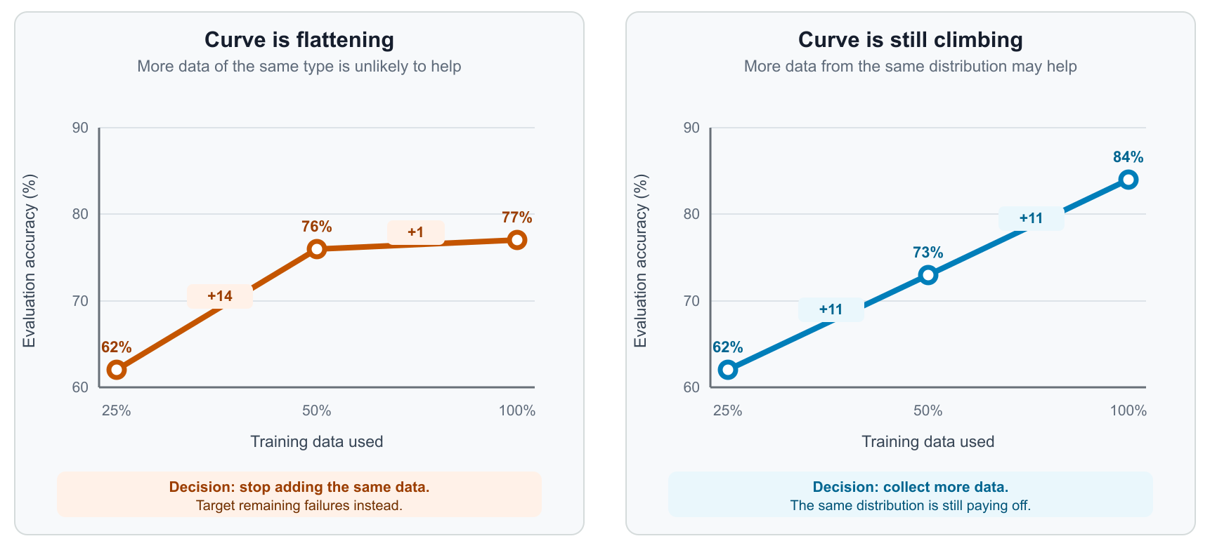
Figure 1: Read the gain from each doubling, not only the final score. When doubling the data improves the primary metric by less than 1 to 2 percentage points, more data of the same type is unlikely to help. Values are illustrative
Why more data doesn’t always mean better performance
SFT doesn’t follow the same monotonic power-law scaling as pretraining. SFT scaling research shows that data volume alone doesn’t guarantee proportional gains. What matters is coverage and depth of the instruction set. Data Repetition Beats Scaling demonstrated this strikingly. Under a fixed compute budget, 128 epochs on 400 reasoning examples beat single-epoch training on 51,200 examples by 12–26 percentage points on AIME and GPQA. A smaller, high-quality dataset trained to full memorization can outperform a larger dataset the model sees only once. Training token accuracy serves as a practical stopping criterion, because gains plateau after the model achieves near-perfect training accuracy.
Data subset selection and filtering
When diminishing returns set in, intelligent data selection can outperform training on the full set. Methods like DEITA, DELIFT, and coreset selection identify the smallest subset that covers your task space while maintaining quality and diversity. These methods score candidates on quality, diversity, and how much each example actually teaches the model. Two benefits stand out:
- Matching or exceeding full-data performance with fewer samples. Removing redundant or low-quality examples provides cleaner gradient signal. AlpaGasus showed that filtering to the top 20 percent by quality trained faster and scored higher than the full set. Rethinking Data Selection demonstrates that subset selection can outperform full-dataset training.
- Reduced catastrophic forgetting. Fewer, more targeted samples mean fewer gradient updates pulling the model away from its pretrained capabilities. This makes subset selection a natural complement to data mixing: you get task specialization with less forgetting, potentially reducing the need for mixing at all.
A practical workflow ties readiness evaluation and selection together. The learning curve is a diagnostic (one training run with saved checkpoints), so you reach these decisions without repeated full-scale training runs:
- Run the learning-curve diagnostic on your full dataset.
- Identify the saturation point.
- If it saturates early, the tail of your dataset is adding little signal. Curate a high-value subset (quality and diversity filtering) and make that your training set going forward. This is not repeating the diagnostic run for the same result: a curated subset trains faster on every future retraining cycle, and quality filtering often scores higher than the full set by removing low-value examples that add noise to the gradient (the AlpaGasus result cited earlier in this section).
- If it’s still improving at 100 percent, data volume is the bottleneck. Collect more data targeting failure cases from error analysis, not more of the same distribution.
- If targeted data is expensive, consider reinforcement fine-tuning with programmatic verification as a more efficient path.
Data augmentation
When your dataset is too small or too narrow, augmentation can expand it without proportional annotation cost. The most impactful form of augmentation for modern SFT is generating reasoning traces and synthetic demonstrations. In practice, most teams source augmented data one of three ways:
- Distill from a stronger model. Generate traces or responses from a capable teacher such as DeepSeek-R1 or a frontier commercial model, verify the final answer, and keep the outputs on correct samples. This is how most open reasoning datasets are built.
- Self-generate and filter. Have the base model you’re fine-tuning produce multiple candidate responses per problem at high temperature, then keep only those whose final answers are correct or whose reasoning is self-consistent across samples. This is the core idea behind STaR.
- Amplify human-authored data for high-stakes domains. When correctness matters more than volume, in medical, legal, or safety-critical settings, expert-written examples remain the gold standard. You can amplify them by using a large language model (LLM) to paraphrase expert reasoning into multiple styles while preserving the logical steps.
Beyond reasoning traces, classic augmentation techniques expand instruction datasets directly. Self-Instruct bootstraps new instruction-response pairs from a small seed set, and Evol-Instruct evolves existing instructions along controlled dimensions such as added constraints or deeper reasoning requirements. Simpler transformations also help: paraphrasing prompts to cover phrasing variation, and reformatting responses to match your target output style. These techniques directly address the coverage and depth properties that predict SFT generalization.
Two quality principles govern augmented data. First, diversity in style matters, not just content. Two correct but differently structured solutions are more useful than two copies of the same solution, a pattern MAmmoTH exploits. Second, verification is non-negotiable. Every augmented example should pass the same quality bar as human-curated data, because synthetic generation is one of the most common sources of duplicates and subtle errors. Apply the deduplication and filtering steps from the first post to augmented data before it enters your training set.
Data mixing patterns
When you fine-tune a model for a specific task, you risk degrading its performance on other capabilities, a phenomenon known as catastrophic forgetting. Data mixing addresses this by blending your target-task data with samples that preserve the model’s existing strengths. For Amazon Nova customization, Amazon Nova Forge supports this pattern, so you can blend proprietary data with Amazon-curated training data at each stage of customization.
An important nuance: Data mixing doesn’t always help your target task. Its primary purpose is to retain general capabilities alongside specialization, and mixing in general data often comes at a direct cost to your domain metrics, because every general-data token displaces a domain-data token. Positive transfer does occur when data sources share underlying reasoning patterns: Qwen2.5-Coder found that a 70:20:10 ratio of code, text, and math outperformed training on 100 percent code, even on coding benchmarks.
Conversely, mixing can hurt when token-length imbalance lets general data dominate the loss: even a 5 percent general-data mix by sample count can represent over 80 percent of gradient signal by token count if its sequences are much longer. Monitor token-level ratios, not just sample-level ratios.
The practical implication: Treat data mixing as an insurance policy for general capabilities, not as a performance booster for your target task.
How data mixing works
Instead of training exclusively on task-specific data, you compose each training batch from multiple data sources with controlled proportions. A typical mix might be 70 percent target task, 20 percent general instruction-following, and 10 percent safety data. Mixing happens at the batch level, so the model sees a consistent distribution throughout training.
A few empirical findings from the SFT-mixing literature are worth knowing before you start experimenting. Dong et al. find that the absolute amount of data per skill drives performance more than the precise ratio between categories, so if a skill is weak, add data for it before rebalancing. Dual-stage Mixed Fine-Tuning shows that training on specialty data first, then on general data mixed with a small fraction of specialty data, outperforms both sequential training (which forgets) and flat mixtures (which interfere). And Cao et al. show that optimal mixtures shift with model size and data budget, so there’s no universal ratio and you should plan to experiment.
Automated mixture optimization
When you have many candidate data sources and can’t afford to sweep all combinations manually, automated methods find near-optimal weights with a fraction of the compute. DoReMi trains a small proxy model and up-weights the domains with the highest excess loss, and the resulting weights transfer reliably to full-scale runs. RegMix fits a regression that predicts performance from mixture weights across many small training runs, which is useful when you care about specific downstream benchmarks. Dynamic Data Mixing adjusts weights during training based on how much each source is still contributing, and typically outperforms the best static mixture by 2–5 percent.
| Scenario | Recommended approach |
| 2–3 data sources, clear priority | Manual: try 3 fixed ratios, pick the best |
| Over 5 sources, unclear interactions | RegMix: fit a regression from 50 small runs |
| Large-scale training, budget for proxy | DoReMi: train a small proxy to find weights |
| Repeated training runs, evolving data | Dynamic: adjust weights during each run |
For most practitioners starting out, the manual approach is sufficient: pick 3–5 candidate mixtures reflecting different priorities, train each for a short run, evaluate, and scale the winner up. Graduate to automated methods when you have more than five data sources or run regular retraining cycles.
Choosing your mix ratio
There’s no universal optimal ratio. As a rule of thumb, the more specialized the task, the more target-heavy the mix: highly specialized tasks such as medical coding can run 80 percent target data, while light adaptations such as tone changes benefit from closer to an even split, with 5 to 10 percent safety data in either case.
Experiments with Amazon Nova models show a 50/50 split provides a strong balance between specialization and capability retention. Three other findings worth carrying into your own experiments:
- Include the reasoning-instruction-following category. It significantly improves general benchmark performance.
- Watch the learning rate. SFT with data mixing is sensitive to it, so use the defaults of 1e-5 for Low-Rank Adaptation (LoRA) and 5e-6 for full-rank as starting points.
- For multimodal datasets, keep video above 20 percent. This helps maintain general benchmark performance.
Decision framework: mix or don’t mix?
Most customers fine-tune an instruction-tuned model (such as Amazon Nova Lite 2.0 or any off-the-shelf chat model), which has already been post-trained to follow instructions, hold conversations, and respond safely. This framework assumes that starting point. The rare exception is starting from a base checkpoint that has only been pre-trained on next-token prediction. In that case, always mix, because there’s no instruction-following or safety behavior to preserve. From an instruction-tuned starting point, train briefly without mixing and evaluate checkpoints. The decision comes down to two questions, both answered by that single run:
- Does the no-mix run overfit your target data? Watch the signals: training loss keeps falling while validation loss stalls or rises, or target-task validation performance peaks at an intermediate checkpoint and then degrades. Small datasets of a few thousand examples raise this risk, but there is no hard threshold. It depends on epochs, learning rate, and whether you train LoRA or full-rank. Respond with training-configuration fixes first: fewer epochs, earlier stopping, a lower learning rate. If overfitting persists, mixing in general data adds gradient diversity and can act as a further regularizer.
- Did the same run regress the general skills you need? Evaluate the capabilities your application needs in production, such as instruction following, conversation, or math and coding. If they held steady, ship without mixing and save the training cost. If they regressed beyond your tolerance, add mixing and scale the general-data ratio to the severity of the regression.
Dataset size and diversity alone don’t settle either question. A 20,000-example medical dataset, however diverse within its domain, can still erode math or coding skills if your application depends on them. That’s why the framework measures instead of assumes.
Data mixing isn’t the only way to fight forgetting. If you update the model repeatedly over time, algorithmic approaches such as OSFT restrict each training run to directions in weight space that don’t disturb prior knowledge. OSFT is available as a drop-in option in Hugging Face PEFT.
Conclusion
The advanced strategies covered here share a common thread: measure before you act. Learning curve analysis tells you whether more data will help. Subset selection tells you which data matters. Augmentation fills gaps that collection can’t reach economically. And a controlled mixing experiment tells you whether capability retention is worth the training cost. Teams that treat these as empirical questions, rather than applying defaults, consistently get better models for less compute.
If you haven’t read it yet, the first post in this series covers the foundations: data quality checks, formatting requirements, and train/evaluation splits.
To get started, visit the Amazon Bedrock console to explore model customization options. Learn more about Amazon Nova on the service detail page, review the Amazon Nova documentation for customization guides, and explore the Amazon SageMaker HyperPod recipes repository for ready-to-run training configurations. For related reading, see Customize Amazon Nova models with Amazon Bedrock fine-tuning on the AWS Machine Learning Blog.
About the authors