Without the ability to track machine learning (ML) model prediction quality, organizations only realize they have issues when their customers complain or when they conduct spot checks, which jeopardizes customer trust. This post introduces inference meta-monitoring for Amazon SageMaker AI endpoints. It provides a governance layer that sits above production ML inference pipelines to continuously track prediction and data quality metrics and visualize trends. You will learn how to design and implement an inference meta-monitoring system specifically for predictive models, using Amazon Quick and optionally with Amazon SageMaker AI MLflow App. The system includes drift detection, delayed ground truth data integration, and automated performance dashboards.
The inference monitoring gap
Developing predictive ML models is often a resource-intensive process. You invest months building training pipelines to drive strong validation accuracy for use cases such as fraud detection, credit scoring or demand forecasting. The performance of the models you deploy might silently degrade, and your teams might notice it only weeks later. Fraud case handlers start to see false positives spiking, and loan officers start to see more applications that should have been previously flagged. Corporate resource planners find themselves with excess inventory because of overestimated demand forecasts.
ML teams therefore need a system that provides them with continuous feedback on the performance of their models in production. The system should immediately alert them whenever model quality or data drift is detected. Teams can then take action early so that model performance remains consistent over time, and customer trust remains high.
Solution overview
This inference meta-monitoring solution combines AWS managed services (Amazon SageMaker AI, Amazon Athena, AWS Lambda, Amazon EventBridge, Amazon Quick) with open source ML tools (SageMaker AI MLflow Apps, Evidently AI).
Prerequisites
- AWS account.
- Use the CloudFormation template provided in the repo to create the virtual private cloud (VPC), subnets, SageMaker AI domain, user profile, and JupyterLab space. The template also clones the git repo and updates the
.envwith the actual values.
Setup
The CloudFormation template automates the entire setup. If you intend to use your existing domains, you can clone the repository, update the env values and run the notebooks in sequence.
Environment setup
Running the CloudFormation setup creates and initializes the variables.

If you intend to use your own SageMaker AI domain, copy over the .env.example to .env and update the file with your specific environment variables. The settings in .env override all other defaults and settings in config.yaml.
Architecture
The system implements integrated training, inference, and monitoring pipelines, unified through a central Athena Iceberg table, Amazon Quick and SageMaker AI MLflow Apps.
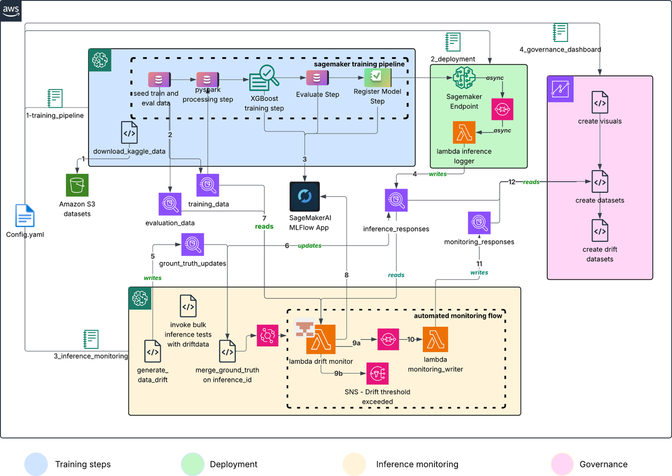
Figure 1: End-to-end MLOps architecture built on AWS managed services
Training (1_training_pipeline.ipynb)
The training pipeline includes experiment tracking in MLflow. As shown in Figure 2, it sets up the end-to-end model training.
1. Download Kaggle dataset: Credit card fraud dataset is downloaded from Kaggle.
2. Data ingestion: S3 data is loaded into the training data. The architecture uses five Athena Iceberg tables to form the central data lake. The training_data table stores the 80% slice the model is fit on. The evaluation_data table is the frozen 20% held-out slice the model is scored on. evaluation_data is the drift-monitoring baseline, not training_data, because the held-out slice is what every registered model’s metrics are measured against. Both tables are populated from the same predictions CSV by a single seed step that applies a deterministic hash split on transaction_id, so the row partition is stable across pipeline runs.
The SeedAthenaTrainingData step (see Figure 2) idempotently loads the predictions CSV from Amazon S3 into the training_data (80%) and evaluation_data (20%) Iceberg tables using a deterministic hash split on transaction_id. Re-runs produce identical row partitions, so the evaluation slice is stable across model versions and usable as a frozen drift baseline. Alternatively, you can replace the training data with your own. For further details, refer to Bring your own dataset.
3. Training: The training and evaluation steps run and log metrics and artifacts to a SageMaker AI MLflow App.
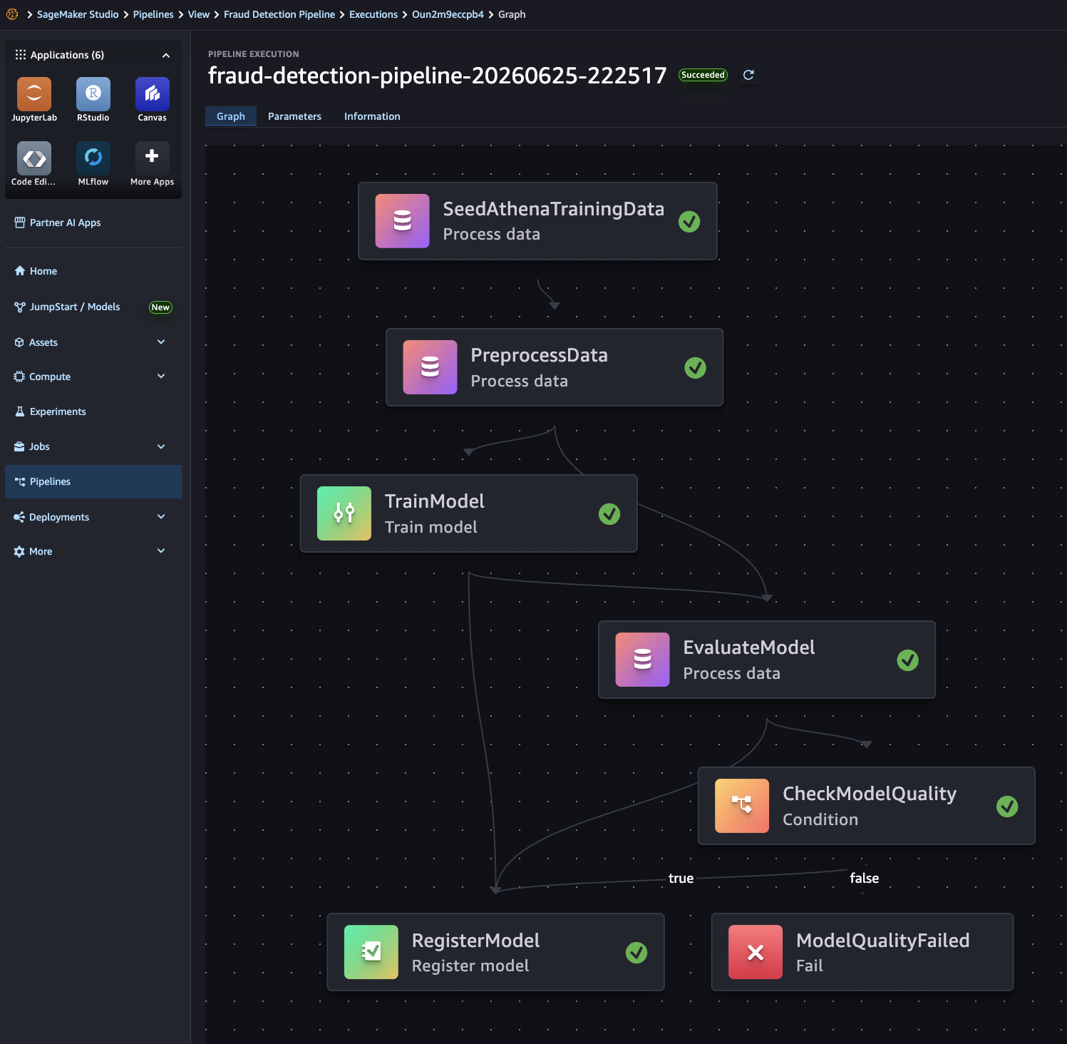
Figure 2: Training pipeline execution
Model deployment (2_deployment.ipynb)
4. Deployment: A custom handler is deployed to a SageMaker AI inference endpoint.
The inference handler writes all the inferences to Amazon Simple Queue Service (Amazon SQS), which are then processed by an inference-logger Lambda function. The inference-logger Lambda function batches up to 10 predictions, or the number of predictions that arrive within 30 seconds, whichever comes first, and writes into Athena Iceberg tables. All the notebooks also include convenience scripts for role creation and infrastructure creation.
Inference monitoring (3_inference_monitoring.ipynb)
5. Ground truth simulation: Step 3.3 in 3_inference_monitoring.ipynb invokes the deployed model with drifted input features. This infuses data drift. In real environments, this would be your typical business applications that send inference requests with drifted inputs over time. The ground truth simulation is step 4 in the notebook.
Steps 3 and 4 of the solution are meant to be replaced by your business processes, which perform two steps before the data and model drift computations:
a. Step 3: Your applications invoke the endpoint for inference. This triggers the inference endpoint to push the inference request into SQS -> Lambda -> Athena (inference_responses).
b. Step 4: You generate ground truth data. This is the process of concluding if a prediction was right or wrong. In the example use case, it is determining if an inference request was a fraud or non-fraud. In this solution, the ground truth simulation randomly flips the actual field to be fraud/non-fraud, to infuse 15% inaccuracy in model performance. This induces model drift. In real-world scenarios, the actual fraud/non-fraud designation would be made when your fraud team investigates and confirms labels based on auto-approved transactions, customer-disputed chargebacks or a bank confirming fraud/non-fraud cases.
NOTE: Steps 2, 3, and 4 in notebook 3 (generate drifted data, send predictions, apply ground truth) are not scheduled operations. They exist only for dev/test purposes. In production you would replace these with your own business processes: applications hitting the endpoint for inference (steps 2-3) and fraud-investigation feeds writing to ground_truth_updates (step 4). To try this solution end-to-end, trigger these three steps via the notebook cells or the CLI scripts provided in the repo.
With steps 2 and 3, inference requests with data drift are already in inference_responses. Step 4 writes records into the ground_truth_updates table. Records with ground_truth = NULL are picked and new records are created in the ground_truth_updates table with actual labels. With this we can expect model drift upon computation.
At any point you can validate the records through a query editor of your choice:
Figure 3: Query editor showing the generated records
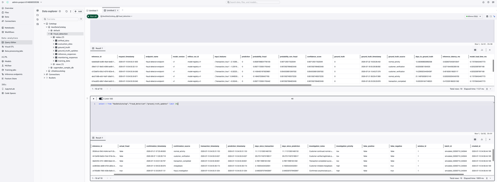
Figure 4: Records in the inference_responses table with ground truth updates and the ground_truth_updates table
Records in the inference_responses table with ground_truth=NULL correspond to the entries for which ground truth hasn’t been applied.
6. Merge ground truth with inference response: Predictions and inference requests captured in the inference_responses table can be joined with ground_truth_updates on inference_id. The inference_responses table captures every prediction along with its features, confidence scores, and timestamps. The ground_truth_updates table holds asynchronous label confirmations that are merged back into inference records through step 4 in the notebook.
Now that we have data to compute data and model drift, we can identify the baseline and current datasets for both categories of computations:
| Metric | Component | Source | ID | Configuration | Example |
| Data Drift | Baseline | training_data | Snapshot_id in iceberg_table also recorded in baseline.json | Automatic during preprocessing step |
If training data had show mean=$500, KS test would flag this distribution shift. |
| Current | Inference_responses for the lookback window | records where request_timestamp >= rolling time window |
Drift lambda env var: DATA_DRIFT_LOOKBACK_DAYS: 1 # Query last 1 days of inferences DATA_DRIFT_THRESHOLD: 0.2 # Alert if ≥20% features drifted |
||
| Model drift | Baseline | Evaluation_data | Snapshot_id in iceberg_table and also recorded in baseline.json | Automatic during preprocessing step |
Lambda queries predictions from last 30 days that have ground truth labels, calculates Lambda queries predictions from last 30 days that have ground truth labels, calculates current ROC-AUC. If baseline was 0.92 and current is 0.85, ROC-AUC degradation = 0.07 (exceeds 0.05 threshold) → Alert! 0.05 threshold) → Alert! |
| Current | Inference_responses with | records where request_timestamp >= rolling time window |
Drift lambda env var: MODEL_DRIFT_LOOKBACK_DAYS: 1 – set to 1 day in deploy_lambda_container.sh because the Lambda is on a daily schedule. Change this value based on how quickly ground truth arrives in your business processes. The config.yaml default is 30 days (for the notebook-driven flow, where a longer window is appropriate because ground truth is often delayed). |
||
Note: If you intend to have a shorter window for drift computations, follow the steps detailed in Configuring Shorter Drift Windows (Minutes instead of days)
The monitoring_responses table stores outputs from the drift computations, including the ModelPackage ARN and Iceberg snapshot ID the run was computed against, so trends can be sliced per model version.
Every registered model carries a frozen baseline.json artifact that records the metrics it earned on evaluation_data, the Iceberg snapshot ID of that exact data slice, and the code commit SHA that produced it. The drift Lambda dereferences these pointers on every run, so the monitoring system always compares production against the precise version of the data and code the deployed model came from, ensuring there is never a stale or wrong-version reference. The lineage mechanism is described in detail in the deep dive section that follows.
7. Drift computation: The drift Lambda function resolves the model currently served by the endpoint and loads its registered baseline.json. Two independent checks run on each invocation, each against its own frozen baseline. For data drift, the frozen training_data slice (pinned through training_snapshot_id in baseline.json) is the reference distribution the model was trained on. Recent inference_responses.input_features from the rolling window is the current distribution. Evidently’s DataDriftPreset compares the two, auto-selecting a statistical test per column. It uses the Kolmogorov-Smirnov or Chi-square (p-values) for smaller samples, and Wasserstein or Jensen-Shannon distances for n ≥ 1000. For model drift, the frozen evaluation_data slice (pinned through evaluation_snapshot_id) supplies the baseline (target, prediction) pairs the model was scored on at training time. Current inference rows joined with ground_truth_updates are compared to that baseline via Evidently’s ClassificationPreset, which tracks ROC-AUC, precision, recall, and F1 degradation. Both baselines are immutable per model version, so re-seeding the source tables later cannot retroactively change historical drift comparisons. Because Evidently emits raw scores whose drift direction depends on the chosen test (p-values: lower = drift. Distances: higher = drift), the solution also computes a normalized companion field, drift_magnitude, so features can be compared and ranked test-agnostically. Follow the drift story for deeper insight into the metrics.
NOTE: Two additional tables are created but not currently used. The ground_truth table holds confirmed labels (fraud/not fraud) and is reserved as a placeholder to update the baseline data for cases where the model has been retrained and you would like to add additional data to the baseline. The drifted_data table is created as a placeholder to contain drifted datasets if needed.
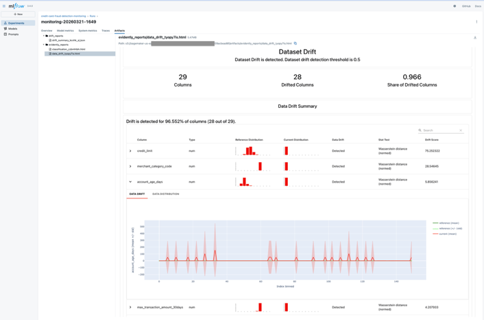
8. Drift logging: The drift monitor Lambda function uses Evidently to generate interactive charts which get logged to SageMaker AI MLflow App. You can also choose to use only Amazon Quick for all your analytics. This solution provides both MLflow with Evidently and Amazon Quick support to cater to both data scientists and governance personas.
9. Monitoring automation: The drift monitor Lambda function checks drift thresholds and triggers alarms if the thresholds are exceeded.
10 – 11. The drift monitor Lambda function also pushes the computations to Amazon SQS and the Lambda writer reads the results and writes the output to the monitoring_responses table. Since the solution uses Apache Iceberg based Athena tables, updates are ACID-compliant.
Meta-monitoring (4_governance_dashboard.ipynb)
12. Governance dashboard: The solution includes a pre-built Amazon Quick analysis with three sheets and 32 visuals querying the Athena monitoring_responses table. Model Drift Trends (11 visuals) shows ROC-AUC degradation, classification metrics, and run counts sliced by model version and training snapshot. Data Drift Trends (10 visuals) shows drifted_columns_share over time, drift-detected verdict rate, and correlation with inference volume. Feature Drift Trends (11 visuals) ranks features by drift_magnitude (test-agnostic “× past threshold” – 1.0 = at threshold, ≥3.0 = severe), with heatmaps of feature × time and feature × model version, and a repeat-offender chart. Two additional visuals split the raw drift_score by test family (p-value tests on one, distance tests on the other) so readers can audit the underlying statistic on its own scale, with sheet-scoped filter groups on drift_method to keep the axes honest. Severity color-coding uses categorical bands (Low <1.0 / Moderate ≥1.0 / Significant ≥3.0) computed from drift_magnitude in the Athena view, so a red cell means the same thing regardless of which underlying test produced it. Every sheet ends with a raw source-data table for lookup. The following sections show you how to extend the dashboards or build your own using natural language queries.
Deep dive into inference monitoring and meta-monitoring
The following sections break down the inference monitoring and meta-monitoring components in more detail.
Inference monitoring with SageMaker AI MLflow Apps and Evidently AI
This section examines the inference monitoring setup in more detail.
The configuration file (config.yaml) has defaults with which the solution runs end to end.
MLflow and Athena logging. Monitoring outputs are co-located with training metrics in the SageMaker AI MLflow App. In addition, metrics are written to Amazon SQS which persists them into Athena for governance:
- Metrics: drifted_columns_count, drifted_columns_share, per-feature drift_score_* (raw test statistic, where direction depends on which test Evidently picked), per-feature drift_magnitude_* (test-agnostic “× past threshold”, higher = more drift, used for ranking and thresholding), current_roc_auc, roc_auc_degradation_pct. The monitoring_responses.per_feature_drift_scores JSON column stores {score, magnitude, method, threshold} per feature so downstream dashboards can pick either view.
- Artifacts: Interactive Evidently HTML drift reports, classification reports, and JSON summaries.
- Flags:
data_drift_detectedandmodel_drift_detectedbooleans for automated decision-making.
Reading the drift numbers: drift_score compared to drift_magnitude
Left to its defaults, Evidently auto-selects a drift test per column by type and sample size, so the raw drift_score on monitoring_responses.per_feature_drift_scores would mean opposite things across features in the same run: a KS-tested feature at 0.001 is severely drifted (p-values: lower = drift), while a Wasserstein-tested feature at 0.001 is not drifted at all (distances: higher = drift). Worse, drift_magnitude for a p-value test is threshold / p_value, which is unbounded – at the 5k–10k sample sizes the daily Lambda pulls, KS is hypersensitive, so a trivial difference yields a near-zero p-value and an inflated magnitude.
So, this solution pins one bounded distance metric for every column, Jensen-Shannon distance (range [0, 1], higher = more drift) for both numeric and categorical features, flagged as drifted above DRIFT_THRESHOLD = 0.1, set via DataDriftPreset(num_method=…, cat_method=…, num_threshold=…, cat_threshold=…) in evidently_reports.py. Jensen-Shannon gives every feature the same 0-to-1 “how different is today’s data from training data” score, so you can rank features against each other on one honest scale instead of comparing numbers that mean different things. Test choice is therefore deterministic rather than sample-size-dependent, drift direction is uniform, and the normalized companion field drift_magnitude = score / threshold is bounded to [0, 10]: 1.0 means “at threshold”, > 1.0 means “drifted”, and higher always means more drifted.
Amazon Quick aggregates, Amazon Simple Notification Service (Amazon SNS) alert text, and MLflow ranking all use magnitude. The raw score and the test method are retained for audit.
 |
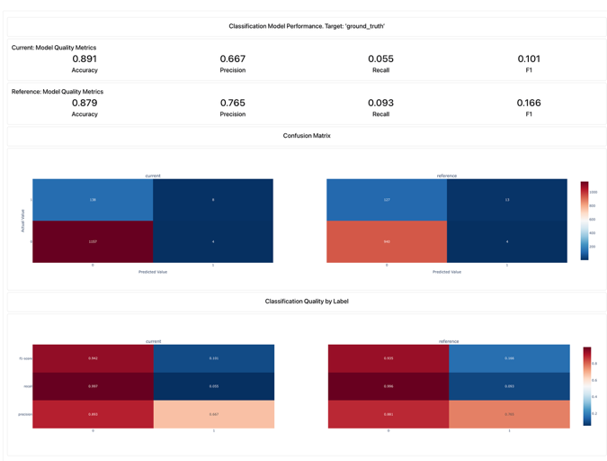 |
Figure 5: Interactive Evidently data drift and classification reports logged in the SageMaker AI MLflow App
Alerting and dashboards. When drift exceeds thresholds, Amazon SNS sends you alerts with direct links to the interactive Evidently reports in MLflow.
Amazon Quick for drift trend analysis
Amazon Quick reads from Athena tables which host the drift computations. Running through the 4_governance_dashboard.ipynb notebook (or the scripts powering it) creates Quick analyses with 3 sheets and 32 pre-built visuals (Model Drift Trends 11, Data Drift Trends 10, Feature Drift Trends 11). Quick also provides calculated fields and natural-language query support for building additional visuals. The pre-built set is a starting point, not a ceiling. If you do not have Amazon Quick set up on your account, follow the README to enable Quick before proceeding with notebook 4.
With Amazon Quick, you can build visuals through drag-and-drop and even through natural language. As shown in Figure 6, explore creating dashboards with prompts like:
“Show me a time series chart of the top 5 drifted features over the last 30 days with drift_magnitude on the y-axis, grouped by day. Include a horizontal reference line at magnitude = 1.0 (the drift threshold). Add a second chart below showing daily prediction volume. Highlight days where more than 3 features had magnitude > 1.0 in red.”
Or
“Create a sankey diagram showing how prediction bucket distributions shifted from the baseline week to last week. Show flows from training data buckets (very_low to very_high fraud probability) to current production buckets. Highlight any bucket that changed by more than 10 percentage points in red.”
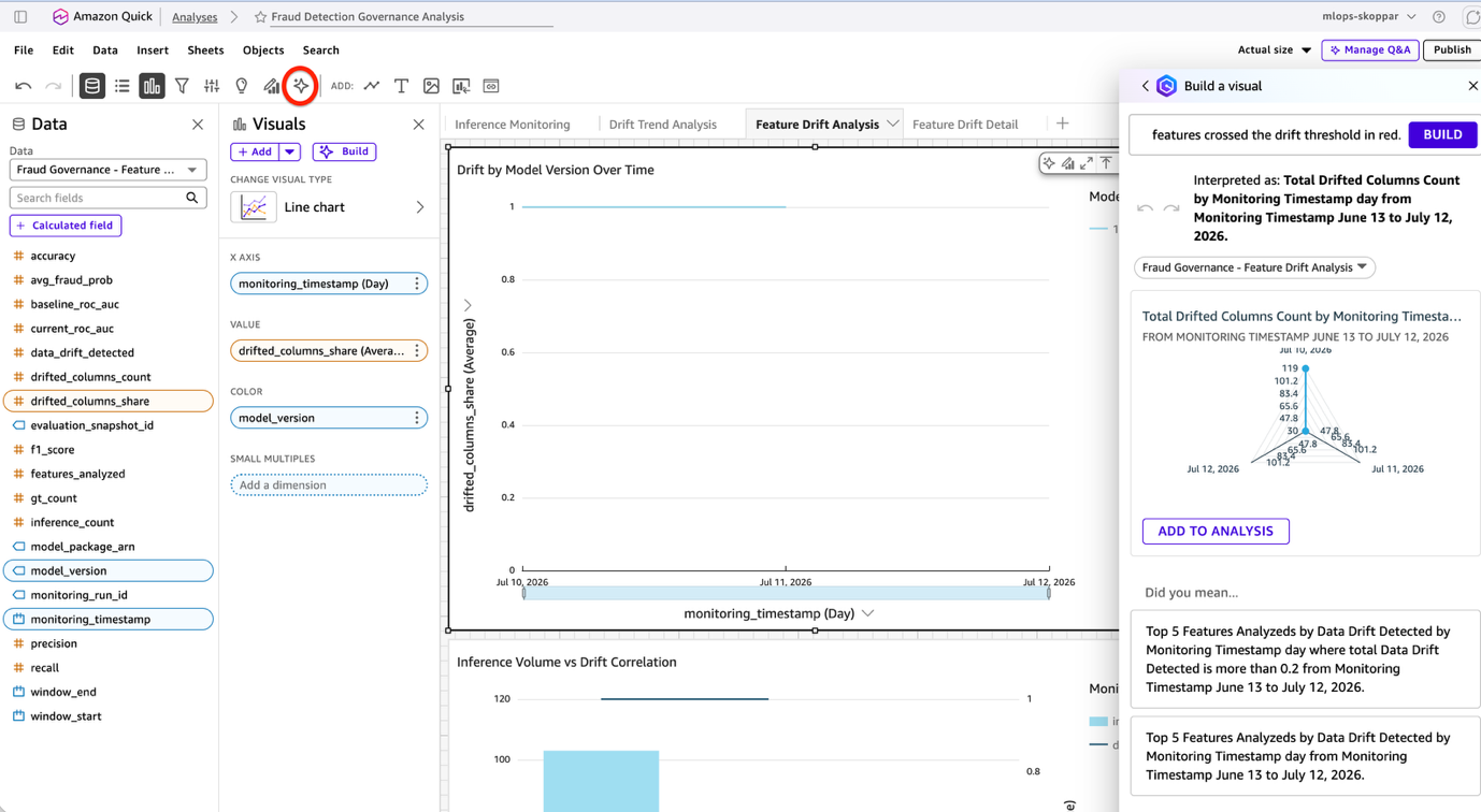
Figure 6: Generate Amazon Quick visuals with natural language
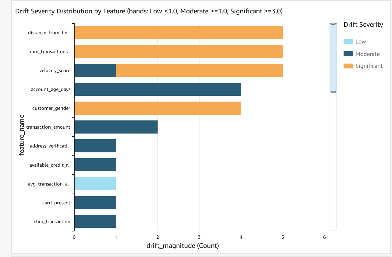
Figure 7: Drift severity distribution by feature. Each horizontal bar shows how many monitoring runs classified the feature as Low (< 1.0), Moderate (≥ 1.0), or Significant (≥ 3.0) drift – bands computed from drift_magnitude, not raw drift_score.
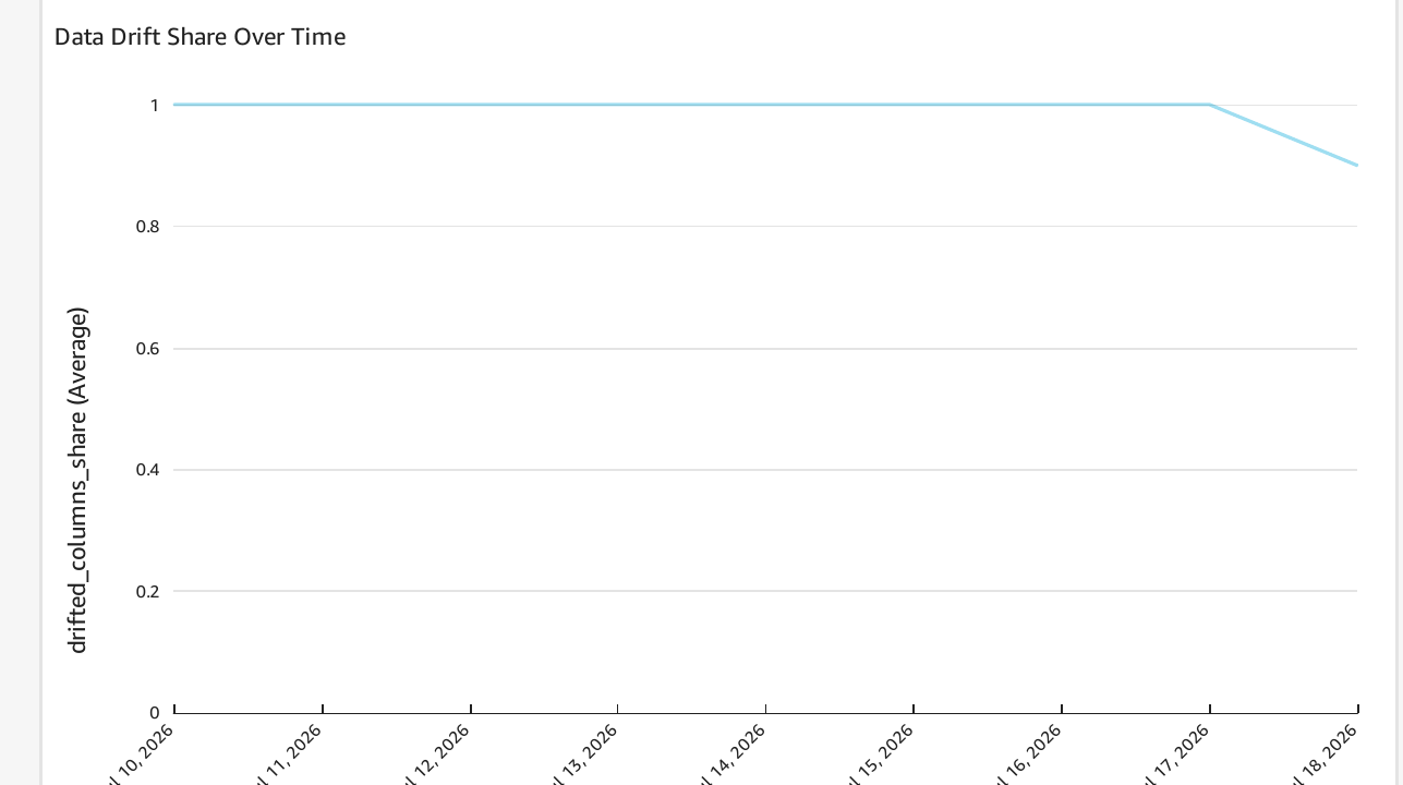
Figure 8: drifted_columns_share sits at 100% for eight straight days (Jul 10-17) before easing to ~90% on Jul 18. Every drift run flagged nearly every feature, well past the 20% alert threshold. The persistence, not the height, is the signal: this is sustained population-wide drift, not a one-day spike.
 |
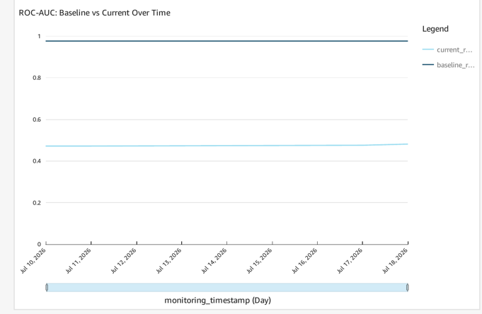 |
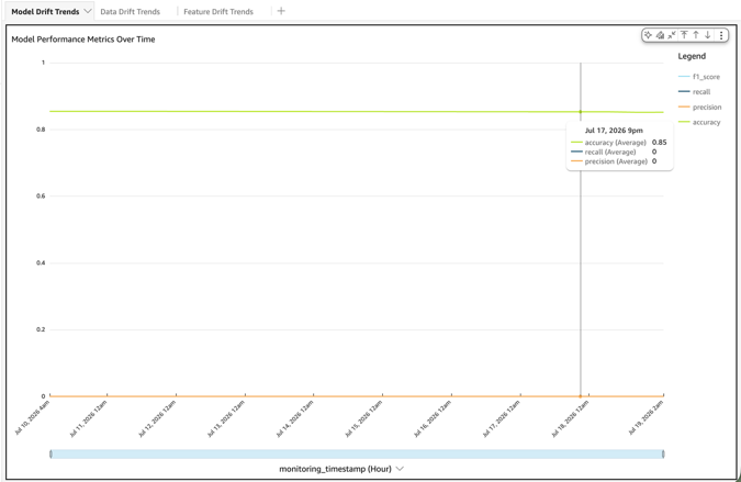
Figure 9: Model drift – Accuracy line (green, ~0.85) stays flat over nine days; precision, recall, and F1 all overlap at 0.0 because the drifted inputs have driven every prediction to the majority class (non-fraud), so TP = FP = 0 structurally. This is exactly why the drift alarm in config.yaml gates on roc_auc_degradation, not accuracy. To the right, Current ROC-AUC (~0.48, light blue) sits flat and ~50 percentage points below the frozen baseline (~0.98, dark blue) across the entire 9-day window, close to random.
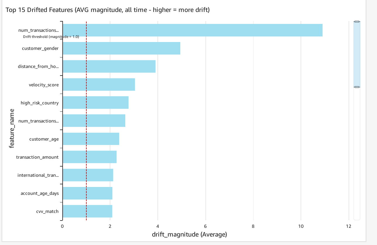
Figure 10: num_transactions_24h leads by a wide margin at ~11× the drift threshold (dashed red line at magnitude = 1.0), with customer_gender, distance_from_home_km, and velocity_score behind at ~5×, ~4×, and ~3× . Every one of the top 15 features sits above the drift line.
Note on the demo screenshots. In these screenshots, the most-drifted feature also happens to be a high-SHAP-importance feature.
 |
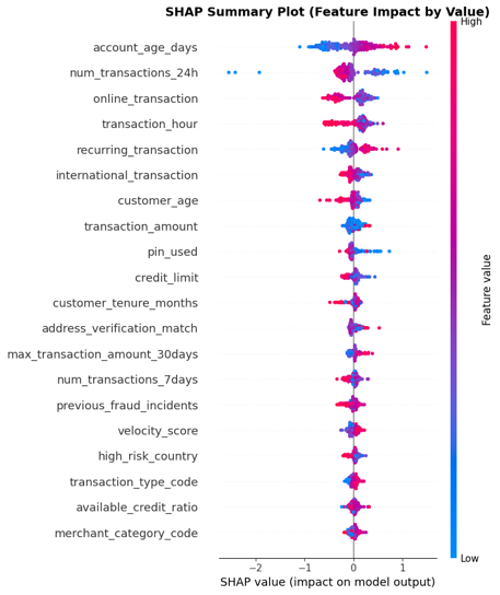 |
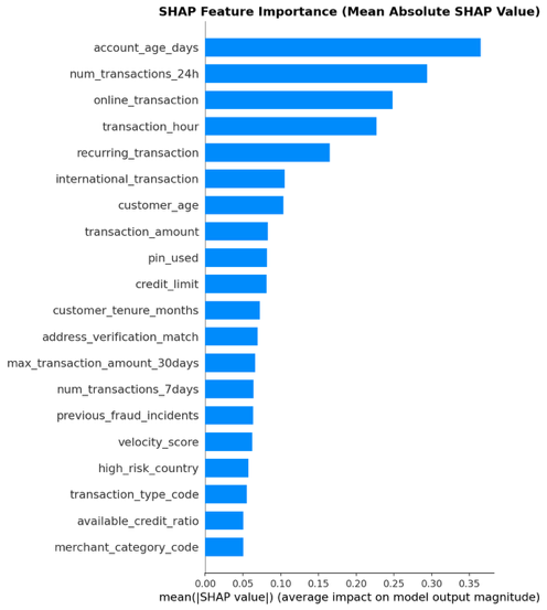
Figure 11: The bar chart shows account_age_days (0.37) and num_transactions_24h (0.29) as the model’s dominant features by mean absolute SHAP, while the beeswarm (right) reveals the direction: red-left / blue-right on account_age_days means older accounts push predictions away from fraud (inverse relationship, matching domain intuition), whereas num_transactions_24h shows a non-monotonic pattern with color mixed at both extremes.
This alignment is a property of the demo drift configuration (config.yaml deliberately drifts a PCA component the model relies on), not something Quick discovered, because it only visualizes Evidently’s statistical distances and has no access to the model or SHAP. In real production drift, magnitude and SHAP importance are independent. The recommended pattern is to cross-reference both when prioritizing which drifted feature matters.
Choice of monitoring visualizations
This solution ships two independent monitoring backends, MLflow and Amazon Quick, on top of the same durable Amazon Athena tables. They are peer consumers rather than a stack, so using one does not require the other, and disabling one has no effect on the other. Every drift run writes its verdict, per-feature scores, and lineage references (model package ARN, training and evaluation snapshot IDs, monitoring run ID) directly to the monitoring_responses and inference_responses Iceberg tables.
Amazon Quick reads from Athena (through AWS Lake Formation if enabled) regardless of whether MLflow is running.
Choose by workload
For online endpoint monitoring with real-time or serverless inference for continuously arriving traffic, pick Amazon Quick. Athena-backed dashboards refresh on schedule, slice by model version, endpoint, training snapshot, or feature, and give stakeholder-facing views suitable for model-risk committees and executive reviews. For batch inference monitoring with scheduled transforms, offline scoring, or discrete jobs, pick MLflow or Quick, depending on team preference:
MLflow provides per-run experiment tracking, hyperparameter and metric comparison across runs, and hosts the full interactive Evidently HTML reports as artifacts, which is a natural fit for discrete jobs where each batch is its own experiment.
Amazon Quick still works here if you want a unified dashboard surface across both online and batch workloads. The two backends answer different questions well.
MLflow answers “what changed between this run and the last, and can I open the Evidently HTML to inspect column by column?”,
while Quick answers “what does the last 90 days of drift look like across every model version and endpoint, and can I share that dashboard with compliance?“
Because both consume the same monitoring_responses table, choosing one does not preclude adding the other later, and neither is a prerequisite for the drift-detection pipeline itself. The daily drift Lambda persists its results to Athena unconditionally.
Cost
All compute scales to zero when idle. Serverless endpoints charge only for actual invocations (no baseline instance hours), Lambdas execute on-demand, Athena queries run only when triggered, and Amazon EventBridge incurs no cost between scheduled runs.
Cost optimization: Iceberg table partitioning reduces Athena scan costs by 10-100x, because you can write queries that filter on the partition column, letting Athena skip partitions. Lambda batching (100 records/invocation) minimizes execution charges, and serverless endpoint auto scaling eliminates over-provisioning waste.
The full solution including SageMaker AI MLflow Apps, SageMaker Serverless Inference, Lambda, Amazon EventBridge, Athena, S3, SQS, SNS, and Quick, costs approximately $60 per month depending on instance type and usage patterns. This figure is directional and will vary based on inference volume, data retention policies, and regional pricing. High-volume deployments scale linearly, with no upfront capacity planning or reserved instances required. The cost estimates are based on pricing as of this writing. For the latest prices, check out Amazon SageMaker AI pricing.
Important: This solution creates billable AWS resources. Charges accrue until resources are deleted. Follow the cleanup steps in 6_optional_cleanup.ipynb to make sure that all resources are removed when no longer needed.
Conclusion
Production ML systems require the same rigor for inference that we apply to training. Inference meta-monitoring transforms reactive incident response into proactive governance.
This solution demonstrates that inference monitoring does not require additional managed monitoring-specific services. By combining Amazon SageMaker AI for model hosting, SageMaker AI MLflow Apps for unified experiment and monitoring tracking, Evidently AI for statistical drift analysis, and Amazon Quick for executive dashboards, you can build a comprehensive monitoring system that is cost-efficient and portable.
Next steps
To get started, clone the sample MLOps best practices repository on the GitHub website.
You can then extend it based on your own business needs. For example:
- Multi-model monitoring: Track multiple endpoints/models from a single monitoring infrastructure, comparing drift patterns across models.
- Automated retraining triggers: Connect the drift alerts to a SageMaker Pipeline that automatically starts retraining when drift exceeds a sustained threshold (not just a single spike).
- Custom drift metrics: Add domain-specific drift tests beyond Evidently’s default per-column tests and classification metrics, such as business KPIs like approval rate shifts, dollar-value impact of false positives, or population-stability metrics on business-critical segments. The drift_magnitude normalization (“× past threshold”) makes it easy to plug in a custom test alongside Evidently’s built-in tests. Because magnitude is universal, downstream ranking still works.
About the authors