With a wide array of Nova customization offerings, the journey to customization and transitioning between platforms has traditionally been intricate, necessitating technical expertise, infrastructure setup, and considerable time investment. This disconnect between potential and practical applications is precisely what we aimed to address. Nova Forge SDK makes large language model (LLM) customization accessible, empowering teams to harness the full potential of language models without the challenges of dependency management, image selection, and recipe configuration. We view customization as a continuum within the scaling ladder, therefore, the Nova Forge SDK supports all customization options, ranging from adaptations based on Amazon SageMaker AI to deep customization using Amazon Nova Forge capabilities.
In the last post, we introduced the Nova Forge SDK and how to get started with it along with the prerequisites and setup instructions. In this post, we walk you through the process of using the Nova Forge SDK to train an Amazon Nova model using Amazon SageMaker AI Training Jobs. We evaluate our model’s baseline performance on a StackOverFlow dataset, use Supervised Fine-Tuning (SFT) to refine its performance, and then apply Reinforcement Fine Tuning (RFT) on the customized model to further improve response quality. After each type of fine-tuning, we evaluate the model to show its improvement across the customization process. Finally, we deploy the customized model to an Amazon SageMaker AI Inference endpoint.
Next, let’s understand the benefits of Nova Forge SDK by going through a real-world scenario of automatic classification of Stack Overflow questions into three well-defined categories (HQ, LQ EDIT, LQ CLOSE).
Case study: classify the given question into the correct class
Stack Overflow has thousands of questions, varying greatly in quality. Automatically classifying question quality helps moderators prioritize their efforts and guide users to improve their posts. This solution demonstrates how to use the Amazon Nova Forge SDK to build an automated quality classifier that can distinguish between high-quality posts, low-quality posts requiring edits, and posts that should be closed. We use the Stack Overflow Question Quality dataset containing 60,000 questions from 2016-2020, classified into three categories:
HQ (High Quality): Well-written posts without edits
LQ_EDIT (Low Quality – Edited): Posts with negative scores and multiple community edits, but remain open
LQ_CLOSE (Low Quality – Closed): Posts closed by the community without edits
For our experiments, we randomly sampled 4700 questions and split them as follows:
Split
Samples
Percentage
Purpose
Training (SFT)
3,500
~75%
Supervised fine-tuning
Evaluation
500
~10%
Baseline and post-training evaluation
RFT
700 + (3,500 from SFT)
~15%
Reinforcement fine-tuning
For RFT, we augmented the 700 RFT-specific samples with all 3,500 SFT samples (total: 4,200 samples) to prevent catastrophic forgetting of supervised capabilities while learning from reinforcement signals.
The experiment consists of four main stages: baseline evaluation to measure out-of-the-box performance, supervised fine-tuning (SFT) to teach domain-specific patterns, and reinforcement fine-tuning (RFT) on SFT checkpoint to optimize for specific quality metrics and finally deployment to Amazon SageMaker AI. For fine-tuning, each stage builds upon the previous one, with measurable improvements at every step.
We used a common system prompt for all the datasets:
This is a stack overflow question from 2016-2020 and it can be classified into three categories:
 * HQ: High-quality posts without a single edit.
 * LQ_EDIT: Low-quality posts with a negative score, and multiple community edits. However, they remain open after those changes.
 * LQ_CLOSE: Low-quality posts that were closed by the community without a single edit.
 You are a technical assistant who will classify the question from users into any of above three categories. Respond with only the category name: HQ, LQ_EDIT, or LQ_CLOSE.
 **Do not add any explanation, just give the category as output**.
Stage 1: Establish baseline performance
Before fine-tuning, we establish a baseline by evaluating the pre-trained Nova 2.0 model on our evaluation set. This gives us a concrete baseline for measuring future improvements. Baseline evaluation is critical because it helps you understand the model’s out-of-the-box capabilities, identify performance gaps, set measurable improvement goals, and validate that fine-tuning is necessary.
Install the SDK
You can install the SDK with a simple pip command:
The Amazon Nova Forge SDK provides powerful data loading utilities that handle validation and transformation automatically. We begin by loading our evaluation dataset and transforming it to the format expected by Nova models:
The CSVDatasetLoader class handles the heavy lifting of data validation and format conversion. The query parameter maps to your input text (the Stack Overflow question), response maps to the ground truth label, and system contains the classification instructions that guide the model’s behavior.
# General Configuration
MODEL = Model.NOVA_LITE_2
INSTANCE_TYPE = 'ml.p5.48xlarge'
EXECUTION_ROLE = '<YOUR_EXECUTION_ROLE_ARN>'
TRAIN_INSTANCE_COUNT = 4
EVAL_INSTANCE_COUNT = 1
S3_BUCKET = '<YOUR_S3_BUCKET>'
S3_PREFIX = 'stack-overflow'
EVAL_DATA = './eval.csv'
# Load data# Note: 'query' maps to the question, 'response' to the classification label
loader = CSVDatasetLoader(
query='Body', # Question text column
response='Y', # Classification label column (HQ, LQ_EDIT, LQ_CLOSE)
system='system' # System prompt column
)
loader.load(EVAL_DATA)
Next, we use the CSVDatasetLoader to transform your raw data into the expected format for Nova model evaluation:
# Transform to Nova format

loader.transform(method=TrainingMethod.EVALUATION, model=MODEL)
loader.show(n=3)
The transformed data will have the following format:
Before uploading to Amazon Simple Storage Service (Amazon S3), validate the transformed data by running the loader.validate() method. This helps you to catch any formatting issues early, rather than waiting until they interrupt the actual evaluation.
# Validate data format
loader.validate(method=TrainingMethod.EVALUATION, model=MODEL)
Finally, we can save the dataset to Amazon S3 using the loader.save_data() method, so that it can be used by the evaluation job.
# Save to S3
eval_s3_uri = loader.save_data(
    f"s3://{S3_BUCKET}/{S3_PREFIX}/data/eval.jsonl"
)
Run baseline evaluation
With our data prepared, we initialize our SMTJRuntimeManager to configure the runtime infrastructure. We then initialize a NovaModelCustomizer object and call baseline_customizer.evaluate() to launch the baseline evaluation job:
# Configure runtime infrastructure
runtime_manager = SMTJRuntimeManager(
instance_type=INSTANCE_TYPE,
instance_count=EVAL_INSTANCE_COUNT,
execution_role=EXECUTION_ROLE
)
# Create baseline evaluator
baseline_customizer = NovaModelCustomizer(
model=MODEL,
method=TrainingMethod.EVALUATION,
infra=runtime_manager,
data_s3_path=eval_s3_uri,
output_s3_path=f"s3://{S3_BUCKET}/{S3_PREFIX}/baseline-eval"
)
# Run evaluation# GEN_QA task provides metrics like ROUGE, BLEU, F1, and Exact Match
baseline_result = baseline_customizer.evaluate(
job_name="blogpost-baseline",
eval_task=EvaluationTask.GEN_QA # Use GEN_QA for classification
)
For classification tasks, we use the GEN_QA evaluation task, which treats classification as a generative task where the model generates a class label. The exact_match metric from GEN_QA directly corresponds to classification accuracy, the percentage of predictions that exactly match the ground truth label. The full list of benchmark tasks can be retrieved from the EvaluationTask enum, or seen in the Amazon Nova User Guide.
Understanding the baseline results
After the job completes, results are saved to Amazon S3 at the specified output path. The archive contains per-sample predictions with log probabilities, aggregated metrics across the entire evaluation set, and raw model predictions for detailed analysis.
In the following table, we see the aggregated metrics for all the evaluation samples from the output of the evaluation job (note that BLEU is on a scale of 0-100):
Metric
Score
ROUGE-1
0.1580 (±0.0148)
ROUGE-2
0.0269 (±0.0066)
ROUGE-L
0.1580 (±0.0148)
Exact Match (EM)
0.1300 (±0.0151)
Quasi-EM (QEM)
0.1300 (±0.0151)
F1 Score
0.1380 (±0.0149)
F1 Score (Quasi)
0.1455 (±0.0148)
BLEU
0.4504 (±0.0209)
The base model achieves only 13.0% exact-match accuracy on this 3-class classification task, whereas random guessing would yield 33.3%. This clearly demonstrates the need for fine-tuning and establishes a quantitative baseline for measuring improvement.
As we see in the next section, this is largely due to the model ignoring the formatting requirements of the problem, where a verbose response including explanations and analyses is considered invalid. We can derive the format-independent classification accuracy by parsing our three labels from the model’s output text, using the following classification_accuracy utility function.
def classification_accuracy(samples):
    """Extract predicted class via substring match and compute accuracy."""
    correct, total, no_pred = 0, 0, 0
    for s in samples:
        gold = s["gold"].strip().upper()
        pred_raw = s["inference"][0] if isinstance(s["inference"], list) else s["inference"]
        pred_cat = extract_category(pred_raw)
        if pred_cat is None:
            no_pred += 1
            continue
        total += 1
        if pred_cat == gold:
            correct += 1
    acc = correct / total if total else 0
    print(f"Classification Accuracy: {correct}/{total} ({acc*100:.1f}%)")
    print(f" No valid prediction: {no_pred}/{total + no_pred}")
    return acc

print("???? Baseline Classification Accuracy (extracted class labels):")
baseline_accuracy = classification_accuracy(baseline_samples)
However, even with a permissive metric, which ignores verbosity, we get only a 52.2% classification accuracy. This clearly indicates the need for fine-tuning to improve the performance of the base model.
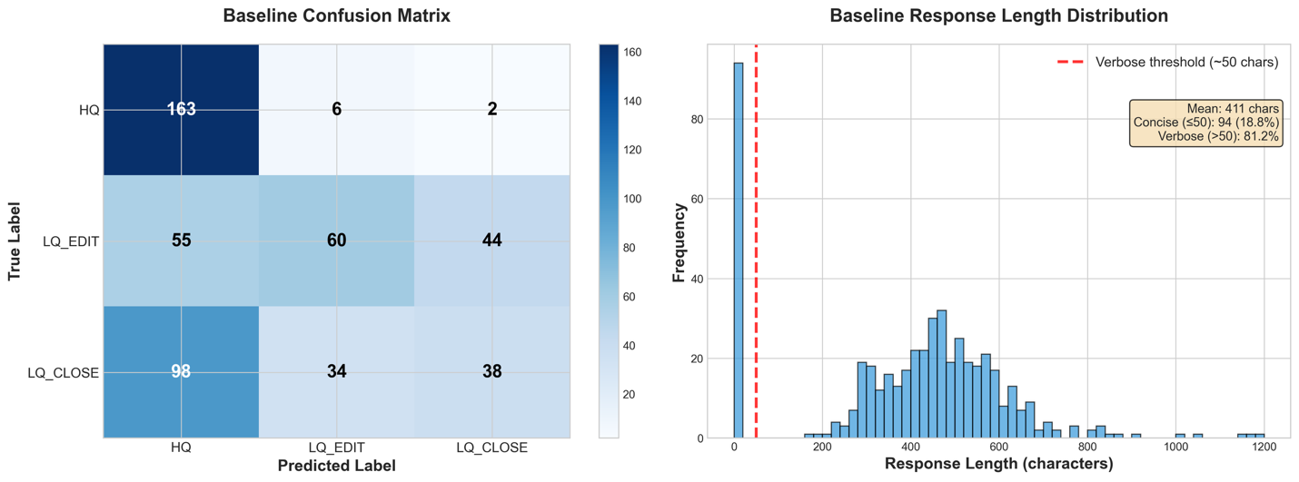
Conduct baseline failure analysis
The following image shows a failure analysis on the baseline. From the response length distribution, we observe that all responses included verbose explanations and reasoning despite the system prompt requesting only the category name. In addition, the baseline confusion matrix compares the true label (y axis) with the generated label (x axis); the LLM has a clear bias towards classifying messages as High Quality regardless of their actual classification.
Given these baseline results of both instruction-following failures and classification bias toward HQ, we now apply Supervised Fine-Tuning (SFT) to help the model understand the task structure and output format, followed by Reinforcement Learning (RL) with a reward function that penalizes the undesirable behaviors.
Stage 2: Supervised fine-tuning
Now that we have completed our baseline and conducted the failure space analysis, we can use Supervised Fine Tuning to improve our performance. For this example, we use a Parameter Efficient Fine-Tuning approach, because it’s a technique that gives us initial signals on models learning capability.
Data preparation for supervised fine-tuning
With the Nova Forge SDK, we can bring our datasets and use the SDKs data preparation helper functions to curate the SFT datasets with in-build data validations.
As before, we use the SDK’s CSVDatasetLoader to load our training CSV data and transform it into the required format:
Now that we have our data well-formed and in the correct format, we can split it into training, validation, and test data, and upload all three to Amazon S3 for our training jobs to reference.
# Save to S3
train_path = loader.save_data(f"s3://{S3_BUCKET}/{S3_PREFIX}/data/train.jsonl")
Start a supervised fine-tuning job
With our data prepared and uploaded to Amazon S3, we initiate the Supervised Fine-tuning (SFT) job.
The Nova Forge SDK streamlines the process by helping us to specify the infrastructure for training, whether it’s Amazon SageMaker Training Jobs or Amazon SageMaker Hyperpod. It also provisions the necessary instances and facilitates the launch of training jobs, removing the need to worry about recipe configurations or API formats.
For our SFT training, we continue to use Amazon SageMaker Training Jobs, with 4 ml.p5.48xlarge instances. The SDK validates your environment and instance configuration against supported values for the chosen model when attempting to start a training job, preventing errors from occurring after the job is submitted.
Next, we set up the configuration for the training itself and run the job. You can use the overrides parameter to modify training configurations from their default values for better performance. Here, we set the max_steps to a relatively small number to keep the duration of this test low.
customizer = NovaModelCustomizer(
    model=MODEL,
    method=TrainingMethod.SFT_LORA,
    infra=runtime,
    data_s3_path=train_path,
    output_s3_path=f"s3://{S3_BUCKET}/{S3_PREFIX}/sft-output"
)

training_config = {
    "lr": 5e-6, # Learning rate
    "warmup_steps": 17, # Gradual LR ramp-up
    "max_steps": 100, # Total training steps
    "global_batch_size": 64, # Samples per gradient update
    "max_length": 8192, # Maximum sequence length in tokens
}

result = customizer.train(
    job_name="blogpost-sft",
    overrides=training_config
)
You can use the Nova Forge SDK to run training jobs in dry_run mode. This mode runs all the validations that the SDK would execute, while actually running a job, but doesn’t start the execution if all validations fail. This helps you to know in advance whether a training setup is valid before trying to use it, for instance when generating configs automatically or exploring possible settings:
result = customizer.train(
    job_name="blogpost-sft",
    overrides=training_config,
    dry_run=True
)
Now that we’ve confirmed the dry_run succeeds, we can move on to launch the job:
result = customizer.train(
    job_name="blogpost-sft",
    overrides=training_config
)
Saving and loading jobs
To save the data for a job that you created, you can serialize your result object to a JSON file, and then retrieve it later to continue where you left off:
# Save to a file
result.dump(file_path=".", file_name="training_result.json")

# Load from a file
result = TrainingResult.load("training_result.json")
Monitoring the Logs post SFT launch
After we have launched the SFT job, we can now monitor the logs it publishes to Amazon CloudWatch. The logs show per-step metrics including loss, learning rate, and throughput, letting you track convergence in real time.
The Nova Forge SDK has built-in utilities for easily extracting and displaying the logs from each platform type directly in your notebook environment.
You can also directly ask a customizer object for the logs, and it will intelligently retrieve them for the latest job it created:
customizer.get_logs(limit=20)
In addition, you can track the job status in real time, which is useful for tracking when a job succeeds or fails:
result.get_job_status() # Returns (JobStatus.IN_PROGRESS, ...) or (JobStatus.COMPLETED, ...)
Evaluating the SFT model
With training complete, we can evaluate the fine-tuned model on the same dataset that we used for baseline evaluation, to understand how much we improved compared to the baseline. The Nova Forge SDK supports running evaluations on the models generated by a training job. The following example demonstrates this:
In the following table, we see the aggregated metrics for the same evaluation dataset after applying SFT training:
Metric
Score
Delta
ROUGE-1
0.8290 (±0.0157)
0.671
ROUGE-2
0.4860 (±0.0224)
0.4591
ROUGE-L
0.8290 (±0.0157)
0.671
Exact Match (EM)
0.7720 (±0.0188)
0.642
Quasi-EM (QEM)
0.7900 (±0.0182)
0.66
F1 Score
0.7720 (±0.0188)
0.634
F1 Score (Quasi)
0.7900 (±0.0182)
0.6445
BLEU
0.0000 (±0.1031)
-0.4504
Even with a short training run, we see improvements in all of our metrics save BLEU (which gives low scores for extremely short responses), going up to 77.2% accuracy for exact match metrics.
print("Post-SFT Classification Accuracy (extracted class labels):")
sft_accuracy = classification_accuracy(sft_samples)
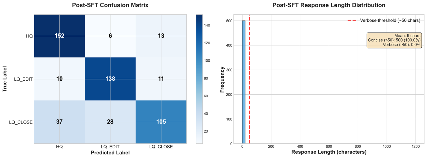
Checking our own classification accuracy metric, we can see 79.0% of evaluation datapoints getting the correct classification. The small difference between classification accuracy and exact match scores shows us that the model has properly learned the required format.
From our detailed performance metrics, we can see that the response length distribution has been pulled fully to non-verbose responses. In the Confusion Matrix, we also see a drastic increase in classification accuracy for the LQ_EDIT and LQ_CLOSE classes, reducing the model’s bias towards classifying rows as HQ.
Step 3: Reinforcement Fine Tuning
Based on the previous data, SFT does well at training the model to fit the required format, but there is still more to improve in the accuracy of the generated labels. Next, we attempt to iteratively add Reinforcement Fine Tuning on top of our trained SFT checkpoint. This is generally beneficial when trying to improve model accuracy, especially on complex use cases where the problem involves more than just fitting a required format and the tasks can be framed in terms of a quantifiable reward.
Building reward functions
For classification, we create an AWS Lambda function that rewards correct predictions with a positive score (+1) and a negative score (-1) for wrong predictions:
1.0: Correct prediction
-1.0: Incorrect prediction
The function handles three quality categories (HQ, LQ_EDIT, LQ_CLOSE) and uses flexible text extraction to handle minor formatting variations in model outputs (for example, “HQ”, “HQ.”, “The answer is HQ”). This robust extraction makes sure that the model receives accurate reward signals even when generating slightly verbose responses. The binary reward structure creates strong, unambiguous gradients that help the model learn to distinguish between high-quality and low-quality content categories.
"""Binary reward function for classification: +1 correct, -1 wrong.
Simple and clear signal:
- Correct prediction: +1.0
- Wrong prediction: -1.0
"""

def calculate_reward(prediction: str, ground_truth: str) -> float:
    """ Calculates binary reward """
    extracted = extract_category(prediction) # Extracts category from prediction and normalize it
    truth_norm = normalize_text(ground_truth) # Normalize the groundtruth

 # Correct prediction
    if extracted and extracted == truth_norm: return 1.0

 # Wrong prediction
    return -1.0

def lambda_handler(event, context):
    """ Lambda handler with binary rewards. """
    scores: List[RewardOutput] = []

    for sample in event:
        idx = sample.get("id", "no_id")
        ground_truth = sample.get("reference_answer", "")
        prediction = last_message.get("content", "")

 # Calculate binary reward
        reward = calculate_reward(prediction, ground_truth)
scores.append(RewardOutput(id=idx, aggregate_reward_score=reward))
return [asdict(score) for score in scores]
Deploy this Lambda function to AWS and note the ARN for use in the RFT training configuration.
Next we deploy the lambda function to AWS account, and get the deployed lambda ARN, so it can be used while launching the RFT training.
Make sure to add Lambda Invoke Policies to your customization IAM role, so that Amazon SageMaker AI can invoke the Lambda policies after training begins.
Data preparation towards RFT
Similarly as the SFT experiment setup, we can use the Nova Forge SDK to curate the dataset and perform validations for RFT schema. This helps in bringing the dataset and transforming them into the OpenAI schema that works for RFT. The following snippet shows how to transform a dataset into RFT dataset.
RFT_DATA = './rft.csv'

rft_loader = CSVDatasetLoader(
    query='Body',
    response='Y',
    system='system'
)

rft_loader.load(RFT_DATA)

# Transform for RFT
rft_loader.transform(method=TrainingMethod.RFT_LORA, model=MODEL)
rft_loader.validate(method=TrainingMethod.RFT_LORA, model=MODEL)

# Save to S3
rft_s3_uri = rft_loader.save_data(
    f"s3://{S3_BUCKET}/{S3_PREFIX}/data/rft.jsonl"
)
After this transformation you will get data in following OpenAI format:
{
    "system": [
        {
            "text": "<system prompt>"
        }
    ],
    "messages": [
        {
            "role": "user",
            "content": [
                {
                    "text": "<input data>"
                }
            ]
        }
    ],
    "reference_answer": "<reference answer>"
    #any other metadata field you use in data loader mapping
}
Launching RFT on SFT checkpoint and Monitoring Logs
Next, we will initialize the RFT job itself on top of our SFT checkpoint. For this step, Nova Forge SDK helps you launch your RFT job by bringing the formatted dataset along with the reward function to be used. The following snippet shows an example of how to run RFT on top of SFT checkpoint, with RFT data and reward function.
We use the following hyperparameters for the RFT training run. To explore the hyperparameters, we aim for only 40 steps for this RFT job to keep the training time low.
rft_overrides = {
    "lr": 0.00001, # Learning rate
    "number_generation": 4, # N samples per prompt to estimate advantages (variance vs cost).
    "reasoning_effort": "null", # Enables reasoning mode High / Low / or null for  non-reasoning
    "max_new_tokens": 50, # This cuts off verbose outputs
    "kl_loss_coef": 0.02, # Weight on the KL penalty between the actor  (trainable policy) and a frozen reference model
    "temperature": 1, # Softmax temperature
    "ent_coeff": 0.01, # A bonus added to the policy loss that rewards  higher-output entropy
    "max_steps": 40, # Steps to train for. One Step = global_batch_size
    "save_steps": 30, # Steps after which a checkpoint will be saved
	"top_k": 5, # Sample only from top-K logits
    "global_batch_size": 64, # Total samples per optimizer step across all  replicas (16/32/64/128/256)
}

# Start RFT training
rft_result = rft_customizer.train(
    job_name="stack-overflow-rft",
    rft_lambda_arn=REWARD_LAMBDA_ARN,
    overrides = rft_overrides
)
We can monitor the RFT training logs using the show_logs() method:
Reward statistics showing the average quality scores assigned by your Lambda function to generated responses.
Critic scores indicating how well the value model predicts future rewards.
Policy gradient metrics like loss and KL divergence that measure training stability and how much the model is changing from its initial state.
Response length statistics to track output verbosity.
Performance metrics including throughput (tokens/second), memory usage, and time per training step.
Monitoring these logs helps us identify issues like reward collapse (declining average rewards), policy instability (high KL divergence), or generation problems (response lengths bumping against the max_token count). After we identify the issues, we adjust our hyperparameters or reward functions as needed.
RFT reward distribution
For the previous RFT training, we used a reward function of +1.0 for correct responses (responses containing the correct label within them) and -1.0 for incorrect responses.
This is because our SFT training already taught the model the required format. If we don’t over-train and disrupt the patterns from SFT tuning, responses will already have the correct verbosity and the model will try to give the right answer (rather than giving up or gaming the format).
We support the existing SFT training by adding kl_loss_coef to slow down the model’s divergence from the SFT-induced patterns. We also limit the max_tokens, which somewhat encourages shorter responses over longer ones (as their classification tokens are guaranteed to be within the window). Given the short training duration, this is sufficient to determine that the RFT tuning represents an improvement in the model’s performance.
Evaluating post SFT+RFT experiment
We use the same evaluation setup as our baseline and post-SFT evaluations to conduct assess our post SFT+RFT customized model. This gives us an understanding of how many improvements we can realize with iterative training. As before, using Nova Forge SDK, we can quickly run another round of evaluation to find the model performance lift.
Results
Metric
Score
Delta
ROUGE-1
0.8400 (±0.0153)
0.011
ROUGE-2
0.4980 (±0.0224)
0.012
ROUGE-L
0.8400 (±0.0153)
0.011
Exact Match (EM)
0.7880 (±0.0183)
0.016
Quasi-EM (QEM)
0.8060 (±0.0177)
0.016
F1 Score
0.7880 (±0.0183)
0.016
F1 Score (Quasi)
0.8060 (±0.0177)
0.016
BLEU
0.0000 (±0.0984)
0
Upon incorporating Reinforcement Fine-Tuning (RFT) into our existing model, we see improved performance compared to the baseline and the standalone Supervised Fine-Tuning (SFT) model. All our metrics consistently improved by around 1 percent.
Comparing the metrics, we see that the order of improvement-deltas is different from that of the SFT fine-tuning, indicating that RFT is calibrating different patterns in the model rather than reinforcing the lessons from the SFT run.
The detailed performance metrics show that our model continues to follow to the requested output format, remembering the lessons of the SFT run. In addition, the classifications themselves are more concentrated on the correct diagonal, with each of the incorrect squares of the confusion matrix showing a decrease in population.
These preliminary indications show that iterative training can help push performance further than just a single training session. With tuned hyperparameters on longer training runs, we could bring these improvements even further.
Final result analysis
Metric
Baseline
Post-SFT
Post-RFT
Delta (RFT-Base)
ROUGE-1
0.158
0.829
0.84
0.682
ROUGE-2
0.0269
0.486
0.498
0.4711
ROUGE-L
0.158
0.829
0.84
0.682
Exact Match (EM)
0.13
0.772
0.788
0.658
Quasi-EM (QEM)
0.13
0.79
0.806
0.676
F1 Score
0.138
0.772
0.788
0.65
F1 Score (Quasi)
0.1455
0.79
0.806
0.6605
BLEU
0.4504
0
0
-0.4504
Across all evaluation metrics, we see:
Overall Improvement: The two-stage customization approach (SFT + RFT) achieved consistent improvements across all metrics, with ROUGE-1 improving by +0.682, EM by +0.658, and F1 by +0.650 over baseline.
SFT vs RFT Roles: SFT provides the foundation for domain adaptation with the largest performance gains, while RFT fine-tunes decision-making through reward-based learning.
BLEU scores are not meaningful for this classification task, as BLEU measures n-gram overlap for generation tasks. Since our model outputs single-token classifications (HQ, LQ_EDIT, LQ_CLOSE), BLEU cannot capture the quality of these categorical predictions and should be disregarded in favor of exact match (EM) and F1 metrics.
Step 4: Deployment to an Amazon SageMaker AI Inference
Now that we have our final model ready, we can deploy it where it can serve real predictions. The Nova Forge SDK makes deployments straightforward, whether you choose Amazon Bedrock for fully managed inference or Amazon SageMaker AI for more control over your infrastructure.
The SDK supports two deployment targets, each with distinct advantages:
Amazon Bedrock offers a fully managed experience with two options:
On-Demand: Serverless inference with automatic scaling and pay-per-use pricing which is perfect for variable workloads and development
Provisioned Throughput: Dedicated capacity with predictable performance for production workloads with consistent traffic
Amazon SageMaker AI Inference provides flexibility when you need custom instance types or specific environment configurations. You can specify the instance type, initial instance count, and configure model behavior through environment variables while the SDK handles the deployment complexity.
We deploy to Amazon SageMaker AI Inference for this demonstration.
This will create the execution role blogpost-sagemaker if it does not exist and use it during deployment. If you already have a role that you want to use, you can pass the name of that role directly.
Invoke endpoint
After the endpoint is deployed, we can invoke it using the SDK. The invoke_inference method provides streaming output for SageMaker endpoints and non-streaming for Amazon Bedrock endpoints. We can use the following code to invoke it:
streaming_chat_request = {
    "messages": [{"role": "user", "content": "Tell me a short story"}],
    "max_tokens": 200,
    "stream": True,}
ENDPOINT_NAME = f"arn:aws:sagemaker:REGION:ACCOUNT_ID:endpoint/{ENDPOINT_NAME}"

inference_result = rft_customizer.invoke_inference(
    request_body=streaming_chat_request,
    endpoint_arn=ENDPOINT_NAME
)
inference_result.show()
Step 5: Cleanup
After you’ve finished testing your deployment, clean up these resources to avoid ongoing AWS charges.
import boto3

iam_client = boto3.client('iam')
role_name = 'your-role-name'

# Detach managed policies
attached_policies = iam_client.list_attached_role_policies(RoleName=role_name)
for policy in attached_policies['AttachedPolicies']:
    iam_client.detach_role_policy(
        RoleName=role_name,
        PolicyArn=policy['PolicyArn']
    )

# Delete inline policies
inline_policies = iam_client.list_role_policies(RoleName=role_name)
for policy_name in inline_policies['PolicyNames']:
    iam_client.delete_role_policy(
        RoleName=role_name,
        PolicyName=policy_name
)

# Remove from instance profiles
instance_profiles = iam_client.list_instance_profiles_for_role(RoleName=role_name)
for profile in instance_profiles['InstanceProfiles']:
    iam_client.remove_role_from_instance_profile(
        InstanceProfileName=profile['InstanceProfileName'],
        RoleName=role_name
    )

# Delete the role
iam_client.delete_role(RoleName=role_name)
Conclusion
The Nova Forge SDK transforms model customization from a complex, infrastructure-heavy process into an accessible, developer-friendly workflow. Through our Stack Overflow classification case study, we demonstrated how teams can use the SDK to achieve measurable improvements through iterative training, moving from 13% baseline accuracy to 79% after SFT, and reaching 80.6% with additional RFT.
By removing the traditional barriers to LLM customization, technical expertise requirements, and time investment, the Nova Forge SDK empowers organizations to build models that understand their unique context without sacrificing the general capabilities that make foundation models valuable. The SDK handles configuring compute resources, orchestrating the entire customization pipeline, monitoring training jobs, and deploying endpoints. The result is enterprise AI that’s both specialized and intelligent, domain-expert and broadly capable.
Ready to customize your own Nova models? Get started with the Nova Forge SDK on GitHub and explore the full documentation to begin building models tailored to your enterprise needs.